Published on
August 10, 2026

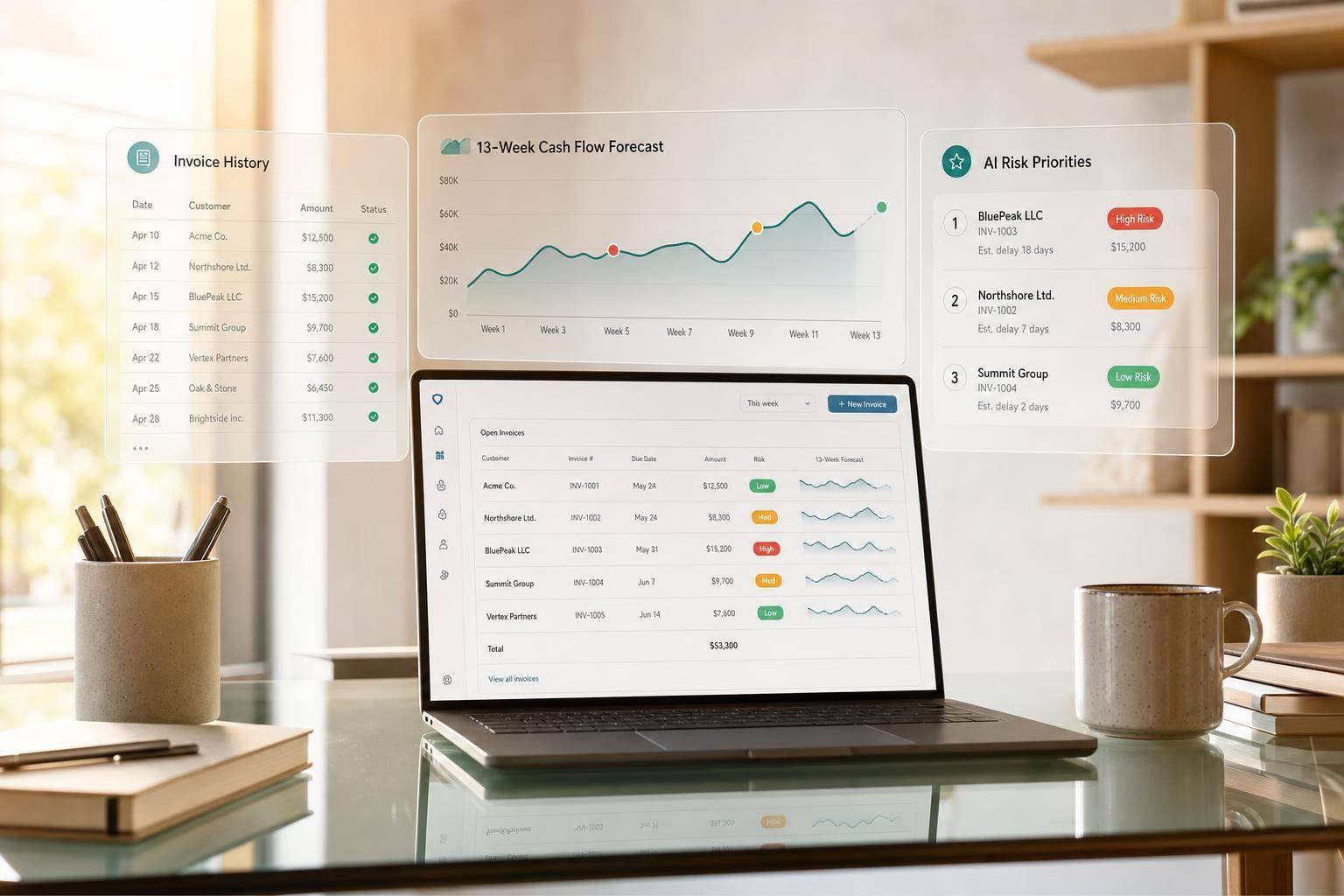
If you wait until an invoice is overdue, you’re already late. I’d sum up this process in one line: use past payment data to score open invoices before the due date, test those scores on older invoices, and tie the results to collection steps and a 13-week cash forecast.
Here’s the short version:
A few numbers make the case. The article notes that nearly 60% of U.S. businesses had invoices more than 30 days overdue, with average unpaid balances of $17,700. It also points out that a workable payment-date model often lands in the 3 to 7 day MAE range for planning, while a false-positive rate under 10% is a common target for higher-touch outreach.
What I like about this approach is that it is not about building a lab project. It is about giving finance teams a simple workflow:
Bottom line: AI late-payment forecasting works when I treat it as a finance process first and a modeling task second.
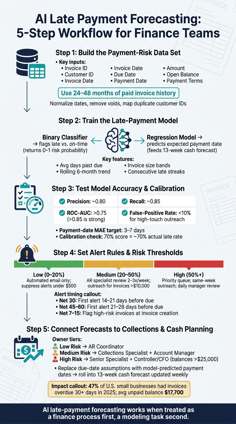
AI Late Payment Forecasting: 5-Step Workflow for Finance Teams
AI forecasts start with clean invoice data. Before a model can flag a risky invoice, your team needs a clean, consistent record of how customers have paid over time.
The model needs invoice-level records that show what you billed and when the customer paid. At a minimum, each invoice record should include the invoice ID, customer ID, invoice date, due date, payment date, invoice amount in U.S. dollars, open balance, and payment terms like Net 30, Net 45, or Net 60.[6][7][9][13]
Past those basics, behavior and collections data can make the model better. Dispute flags, write-off status, partial payment indicators, and logs of earlier collection touchpoints, such as reminder emails or calls, help the model spot the patterns that often come before a late payment.[8][2][10]
It also helps to join customer master data to each invoice. That usually includes legal name, industry, region, account tenure, and any internal credit classification. In many cases, a customer's payment history in your own ledger says more about late-payment risk than external credit scores by themselves.[8][10][13]
Raw AR exports are often messy. The goal is one source-of-truth table with one row per invoice, plus the final amount, due date, paid date, and lateness label.
In practice, that means:
Customer IDs need extra care. ABC Co., A.B.C. Company, and ABC Holdings LLC may all point to the same account. Map them to one canonical ID with a crosswalk table. If you skip that step, the model treats them as different customers. That breaks up payment patterns and hurts accuracy.
You also need one clear definition of late across the full history. Some teams use a simple binary label, where any payment after the due date counts as late. Others use buckets like 1–30 days late, 31–60 days late, or 61+ days late.[1][14]
That cleaned history becomes the training base for the model.
After the history is clean, split it into two groups. Fully paid, closed invoices become the labeled training set because their outcomes are known. Open invoices should stay out of training and get scored only after deployment.[8][9][12]
This matters a lot. If open invoices slip into training, the model learns from data it would not have at prediction time. That can make accuracy look better than it is.
A practical way to handle this is to train on invoices settled before a set date, validate on a later historical window, and then score today's open AR after the model goes live. Use 24 to 48 months of paid invoice history so the model sees enough variation while still reflecting current conditions.[6][9][11]
With the data set in place, the next step is to turn payment history into features the model can score.
Once your AR history is clean and split, the next job is to turn that data into signals the model can learn from. The goal here is simple: build features that reflect how customers behave, not just what appears on an invoice.
The strongest features usually come from past payment behavior. Average days past due is one of the best predictors.[4][17] Add the standard deviation of days late to show how steady or erratic that behavior is. A customer who pays 2 days late one month and 45 days late the next is a bigger risk than one who is consistently 10 days late.[3]
Averages alone don't tell the whole story. Trends matter too. A rolling 6-month average delay, compared with the prior period, shows whether a customer is improving or slipping. You can also add signals like consecutive late-invoice counts, invoice size bands - under $1,000; $1,000–$10,000; $10,000–$50,000; and above $50,000 - and known slow-payment windows such as late December. That matters because some customers pay small invoices on time but drag their feet on larger ones.[4][2][5][18]
There are two practical ways to frame the prediction target.
For many U.S. mid-market businesses, a smart path is to start with the binary model, let the team get comfortable with it, and then add date regression later.
Once the model scores each invoice, finance teams need to know why. A score by itself doesn't help much. The model should give two things for every invoice: a probability of late payment, or a 0–100 risk score, and plain-English reason codes that tell the team what drove that score.[4][7]
For example:
Customer has 4 of the last 6 invoices more than 15 days late.
Invoice amount is larger than this customer's typical size.
Logistic regression and tree-based models can both give finance teams explanations they can use, which is why they show up so often in finance-led AR work.[16][19] That mix of score plus reason codes is what collections and cash planning teams need to decide what to do next.
Before you send scores into collections, test the model hard. If the predictions are off, the damage shows up on live invoices before a collector even has a chance to respond. And here, you’re judging two different outputs from Section 2: late-payment probability and predicted payment date. Each one needs its own check.
After that, you need to see if those invoice scores still work on history the model hasn’t seen before.
Use a time-based holdout so the test looks like live use: train on older invoices, then test on a later period.[3][15][25]
Freeze both the training data and the model as of a set cutoff date. For each invoice in the test period, leave out anything that would not have been known on the invoice date, including later credit changes, disputes, or contract updates. Then compare the model’s predictions with what actually happened.
That setup matters. If the model gets to “peek” at later events, the test looks better than live performance will.
Review the two prediction tracks on their own: one for late vs. not late, and one for payment-date prediction.
For classification, finance teams usually watch precision, recall, ROC-AUC, and false-positive rate.[22][23][24]
| Metric | What It Measures | Practical Target |
|---|---|---|
| Precision | Of flagged invoices, how many actually pay late? | Around 0.80 |
| Recall | Of all late invoices, how many did the model catch? | Around 0.85 |
| ROC-AUC | Overall ability to rank late vs. on-time invoices | Above 0.75; above 0.85 is strong |
| False-positive rate | On-time invoices incorrectly flagged as late-risk | Under 10% for intensive outreach; 15%–20% may be acceptable for low-friction reminders |
In plain terms, precision tells you whether flagged invoices are worth a collector’s time. Recall shows how many late invoices slipped through. ROC-AUC gives you a sense of ranking quality across the whole set. And false-positive rate tells you how often you’re bothering customers who would have paid on time anyway.
For payment-date prediction, use Mean Absolute Error (MAE), measured in days between predicted and actual payment dates.[25][26] An MAE of 3–7 days is workable for most monthly or quarterly cash plans. If the model is still off by more than 10–14 days on a steady basis, add customer-level seasonality, contract renewal cycles, or U.S. holiday schedules to the features, or retrain on more recent data.
Once the timing error is in a good range, check whether the score bands line up with actual late rates.
Calibration means a 70% score should map to about a 70% late rate.[20][21]
To test this, group holdout invoices into score bands such as 0–0.2, 0.2–0.4, 0.4–0.6, 0.6–0.8, and 0.8–1.0, then calculate the actual late rate inside each band. If the scores are not calibrated, alert thresholds become shaky. A “high-risk” cutoff might look clean on paper but fail once the model is in use.
Calibration methods like Platt scaling or isotonic regression can fix this, or you can tune the alert thresholds until the score-to-outcome relationship stays steady across bands.[20][21]
Use those calibrated scores to set the alert thresholds in the next step.
Now that calibration is done, turn those scores into queue rules your collections team can use day to day. The goal is simple: use calibrated scores to build a ranked work queue that tells your team which invoices to touch, when to act, and how to respond before payment turns late.
Start by sorting invoices into three bands based on the model’s late-payment probability score. For many U.S. mid-market businesses, a setup like this works well.[31]
| Risk Band | Score Range | Default Action |
|---|---|---|
| Low | 0–20% | Automated email reminders only; no manual review unless invoice exceeds $50,000 |
| Medium | 20–50% | AR specialist review 2–3 times per week; personalized outreach for invoices above $10,000 |
| High | 50%+ | Priority queue; same-week outreach; daily review with manager review and a clear escalation path |
Probability score on its own doesn’t tell the whole story. You also need to layer in dollar exposure. A common approach is to use a simple priority score: invoice value multiplied by late-payment probability. That helps rank the queue by actual cash impact, not just risk in isolation.[3][34]
If your team is lean, it often makes sense to move the high-risk cutoff up to 65%–70%. That keeps the queue from getting clogged with too many alerts.
Timing matters. If an alert comes too late, the team may not have enough room to change the outcome. Once an invoice is already past due, collection odds drop fast. Some sources put recovery at only 20%–30% once invoices pass 120 days overdue.[30][33]
A practical timing setup by payment terms looks like this.[27][28]
Your alert timing should also match how the team works. If AR reviews queues on Monday, Wednesday, and Friday mornings, batch alerts for those days and have them ready by 8:30 a.m. local time.[27][28]
Even a calibrated model can spit out too many low-value signals if you let every alert through. Two filters help keep the queue usable.
Set invoice-amount minimums first. Suppress high-priority alerts for invoices under $500 unless late risk is above 80% or the customer is already on credit watch. Only show medium-risk alerts in the action queue for invoices above $2,500. High-risk alerts should always appear for invoices above $10,000.[29]
Then add a confidence filter. Only create action-ready alerts when model confidence clears a set floor, such as 70%–80%. If an invoice has a high score but low confidence - often the case with new customers or accounts with little payment history - place it in a “review if time allows” bucket instead of pushing it into the main queue.[31][32] That way, the core queue stays focused on cases where the model has a solid track record.
These rules shape the collections queue. The next step is linking each risk tier to a specific action and a cash forecast.
Use the calibrated risk bands from the last step to assign owners, next steps, and forecast updates. A score means nothing if it doesn't change what the team does.
Each risk band needs a clear owner and a clear next move. If not, scores get ignored or handled differently by different people.
| Risk Tier | Owner | Collection Action | Expected Cash-Flow Impact |
|---|---|---|---|
| Low | AR coordinator | System-generated email; no calls unless invoice exceeds $50,000 | Minor pull-forward; reduces small, unexpected delays |
| Medium | Collections specialist + account manager | Personalized email referencing invoice details; phone call to confirm AP status; early-pay incentive on larger balances | Meaningful DSO reduction; lowers weekly cash-inflow volatility |
| High | Senior collections specialist; controller, VP of Finance, or CFO for balances above $25,000 | Direct calls with customer's finance lead; payment plan negotiation; order holds if needed; leadership-to-leadership outreach on strategic accounts | Major impact on avoiding large, surprise delinquencies; early visibility into potential bad-debt situations |
For high-risk accounts, pull in sales or account management early. That matters more than it may seem. If a collector calls a customer while there's also an active renewal discussion, they need that context. Otherwise, the left hand and right hand can work against each other.
A RACI matrix helps here. Use it to spell out who owns the work, who approves decisions, and who needs to stay in the loop.
Once each tier has a set owner and action, the next step is to turn predicted payment dates into weekly cash buckets.
Due-date forecasting assumes every invoice gets paid on time. In practice, that almost never happens. 47% of U.S. small businesses had invoices overdue by more than 30 days in 2025.[35]
The fix is pretty simple: replace due-date assumptions with model-based expected payment dates at the invoice level, then group those dates into weekly cash buckets. For each open invoice, assign an expected receipt week based on the model's predicted payment date.
From there, split the forecast into low-risk receipts and at-risk receipts. For medium- and high-risk accounts, apply probability weighting. Then roll all of it into your 13-week cash forecast, updating it every week as:
This is where the model starts paying off in day-to-day finance work. Say a $500,000 invoice is likely to slip two weeks past its due date. The team can line up vendor payments differently or draw on a revolving credit line before the gap shows up, not after.
Done well, this workflow turns AR history into earlier collections action and tighter cash forecasts.
Start with clean, consistent data from your ERP, CRM, and banking systems.
The main inputs usually include 12 to 24 months of transaction history, accounts receivable aging reports, and customer payment patterns, including actual payment dates versus invoice dates.
You should also pull in accounts payable, payroll, debt schedules, and tax data. Then standardize everything by removing duplicates and filling in missing values. If the data is messy, the forecast will be too.
It depends on your business goals and the kind of forecasting task you’re dealing with. There’s no one-size-fits-all accuracy target. What matters more is using a model that consistently spots payment patterns that matter without turning into something so complex that no one can explain it or trust it.
A good way to judge performance is to test the model against your liquidity needs with metrics like MAE or MSE. Start simple with a baseline model, then compare its forecasts with actual results each week. If conditions shift, retrain the model so it stays in step with what’s happening.
Predictive scores make a 13-week cash forecast far more responsive because they reflect how customers actually pay. Instead of relying on fixed assumptions, finance teams assign collection probabilities to receivables, such as 85% for current invoices and 20% for invoices that are 90 days overdue.
Pair those scores with automated bank feeds, and the model can adjust fast as payment patterns shift. The result is a clearer view of liquidity, better visibility into risk, and forecast volatility that can drop by as much as 25%.