Published on
August 15, 2026


If I had to boil this down to one point, it’s this: churn drives customer life, customer life drives CLV, and both should shape how I forecast revenue, set CAC limits, and approve retention spend.
Here’s the simple version:
If I’m at a growth-stage company working with a fractional CFO, I don’t need the most advanced model first. I need the simplest model that improves forecast accuracy and spending decisions. In most cases, that means starting with cohort churn and a basic CLV model, then moving to survival, ML, or probabilistic methods only if my data can support it.
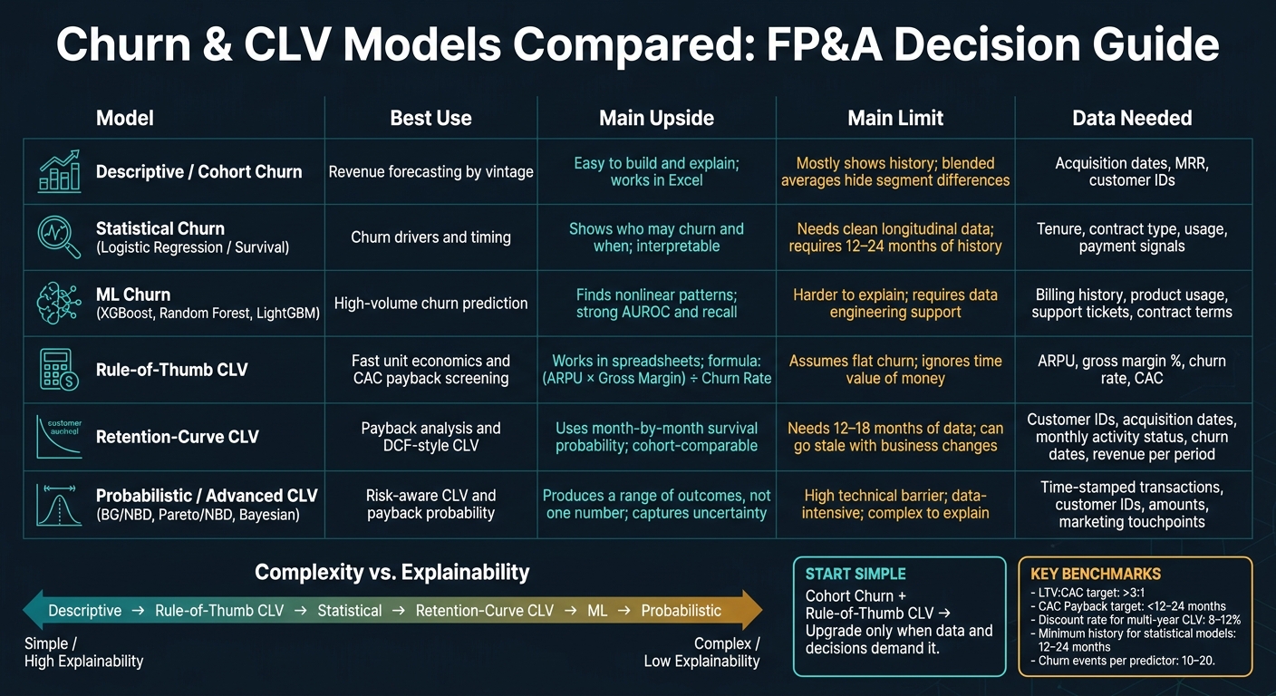
Churn & CLV Models Compared: FP&A Decision Guide
| Model | Best use | Main upside | Main limit |
|---|---|---|---|
| Descriptive / cohort churn | Revenue forecasting by vintage | Easy to build and explain | Mostly shows history |
| Statistical churn | Churn drivers and timing | Shows who may churn and when | Needs clean time-based data |
| ML churn | Higher-volume prediction | Finds nonlinear patterns | Harder to explain and maintain |
| Rule-of-thumb CLV | Fast unit economics | Works well in spreadsheets | Assumes flat churn |
| Retention-curve CLV | Payback and DCF-style CLV | Uses month-by-month survival | Needs more history |
| Probabilistic CLV | Risk-aware CLV and payback | Shows a range, not one number | Harder to build |
What follows is a plain-English look at when each model works, what data it needs, and how I’d use it for forecasts, payback, segment mix, and retention budgets.
Descriptive churn models are the starting point. They show how many customers left and how much revenue disappeared. The main inputs are simple: beginning customers, lost customers, new customers, and MRR. From there, you can calculate logo churn rate, revenue churn rate, and net revenue retention (NRR). Those numbers flow straight into revenue forecasts. For startups scaling quickly, fractional CFO services can help build these models and interpret the results.
Cohort-based models go a step further. They group customers by acquisition date and track how much of each group stays active over time. The result is a cohort retention curve.[2][5][6]
For FP&A, this matters most in forecasting. A blended churn rate can smooth over big differences between customer vintages. Cohort curves show those differences instead of hiding them. That lets FP&A forecast revenue by vintage and then add the cohorts together, rather than applying one churn rate across the full customer base. If customer behavior is changing, that approach usually gives a better forecast.[2][5][6][7]
Cohort models depend on clean acquisition-date data. If that field isn't recorded the same way each time, customers end up in the wrong cohort and the retention curves drift off course. Plan tier, contract value, and acquisition channel also help, because they make segmented curves possible. And those segmented curves are far more useful for planning than one blended view.[2][4][6]
These same curves also help with budget decisions. If one acquisition channel keeps customers longer than another at the same point in the lifecycle, those cohorts support very different CAC limits and payback windows. In plain terms, a customer source with better retention can justify a higher CAC.
Use the curve to set:
When cohort curves still don't explain why churn is happening, statistical models can add driver-level forecasting.
Cohort models tell you what happened. Statistical models tell you why it happened and when it may happen again.
In churn work, that difference matters. Statistical churn models estimate which customers are likely to leave, when they may leave, and which variables push that risk up or down.
A simple rule of thumb helps here:
For FP&A, survival analysis is often the better fit, especially Cox proportional hazards and parametric survival models. These models produce a time-based risk curve, so you can see when churn risk starts to climb instead of squeezing everything into one flat average. In subscription data, the highest churn risk has been observed within the first 20 months after activation. That early-life risk window can disappear inside a blended monthly churn rate.[11]
Survival models produce risk rates that shift over time. FP&A can apply those rates to active customer counts and ARPU to build bottom-up revenue forecasts by segment.
That gives you a much sharper view than a single churn rate for the whole base. An enterprise customer on a multi-year contract may have a 1–2% annual churn probability, while a month-to-month SMB account with weak engagement can run above 25%. Putting those different risk rates on each segment usually leads to a better revenue forecast than using one blended assumption.
Think of it like weather by ZIP code. A national average temperature doesn’t tell you whether to bring a coat in Chicago or sunscreen in Phoenix. Churn works the same way.
These models need clean setup before they can do useful work. You need a clear churn event, steady time stamps, and covariates such as tenure, contract type, pricing tier, usage, payment method, and support signals.
One point trips teams up all the time: customers who are still active at period end should be treated as still at risk, not churned. If that rule gets missed, hazard estimates can drift off course.
You also need enough history. A common guideline is at least 10–20 churn events per predictor, which usually means 12–24 months of data.[11] Without that base, the model may look precise on paper but fall apart in practice.
For FP&A, the payoff is bigger than prediction alone. The point is to turn risk into CLV and payback decisions.
Once the model scores each account, FP&A can convert survival probabilities into expected remaining customer lifetime. From there, those estimates can be combined with expected margin to calculate forward-looking CLV.[12][13] That output feeds straight into payback period analysis by segment or acquisition channel.
On the retention side, hazard ratios from Cox models show how much a variable like contract length, a discount, or an add-on service changes churn risk.[10] That gives finance teams a way to estimate the revenue effect of a retention program before approving spend, instead of going with gut feel.
A particularly useful application is identifying customers with both high churn probability and high ARR, then testing whether a targeted intervention reduces risk enough to justify its cost.
If pricing, product, or customer mix changes fast, retrain the model or use cohort analysis until the pattern settles down.[9][10][11]
When prediction needs higher-dimensional pattern detection, machine learning models go further.
Statistical models help you see why customers leave. ML helps when churn comes from messy signal combinations that don’t follow a straight line. If churn depends on many signals interacting at once, ML can catch patterns that simpler models miss.
These models predict whether a customer will churn within a set time window by blending many inputs at the same time. Tree-based models like XGBoost, random forest, LightGBM, and gradient boosting are often a good fit because they can pick up nonlinear churn patterns. In B2B SaaS, tree-based models such as XGBoost often post strong AUROC and recall. For FP&A, that matters in a very practical way: better recall means fewer at-risk accounts slip through the cracks.
ML can tighten forecasts by giving each customer a churn score, then rolling those scores up into segment-level retention assumptions by plan tier, channel, or segment. That sounds simple enough, but there’s a catch: calibration matters.
If a model gives a customer a 20% churn score, about 20% of customers with that score should end up churning. If that doesn’t hold, the scores may look exact on the surface while still leading to shaky budget forecasts. In other words, a neat-looking score isn’t much help if it points finance in the wrong direction.
ML churn models need solid inputs. The core data usually includes:
One thing can wreck the whole setup: data leakage. That means using information that would not have been available at the time of prediction. It can make test results look far better than they are, then fall apart in production.
Class imbalance is another common issue, so teams often use reweighting or oversampling to deal with it. Clean timestamps matter too. If the timing is off, the model may learn from the future by accident. Before churn scores show up in budget forecasts, the data has to be clean and leakage-free.
The same churn scores that help forecasting can also change CAC limits and retention budgets. Instead of relying on one average churn assumption, ML lets you swap in segment-level retention assumptions based on model scores. That gives finance a sharper view of CAC payback. For example, high-risk early-life cohorts may call for lower CAC caps even if starting ARR looks strong.
On the retention side, the model only earns its keep if it changes what the team does. That usually means deciding which accounts get proactive outreach before renewal and which segments should get more retention budget.
A model that does not change decisions adds noise, not value.
If the scores don’t change outreach plans or spending decisions, a simpler model is the better pick.
Once FP&A has a churn assumption, it can turn that number into a basic CLV estimate. The standard shortcut is (ARPU × gross margin) ÷ churn rate [17][19]. The logic is simple: average customer lifetime is roughly 1 ÷ churn rate. For FP&A teams, that creates a fast link between churn and unit economics by segment.
This model works best when retention is stable and segment mix doesn’t move much. If cohort behavior starts to split, the math gets shaky.
For example, if enterprise and SMB customers keep very different retention patterns, a blended average can distort both groups [22]. The model also leaves out the time value of money, which means it can overstate value across multi-year periods. For multi-year CLV, practitioners recommend using a discount rate between 8% and 12% [1][20].
Use this model for rough payback math. Don’t lean on it for segment-level budgeting.
Its main job is quick CAC payback analysis. At a minimum, you need:
If you also want to check CAC payback, add customer acquisition cost. The good news is that this model fits easily into spreadsheets or basic FP&A dashboards [17][21].
FP&A teams often use this model to ground CAC payback discussions. Here’s the simple version: at $100 in monthly revenue and a 70% gross margin, monthly gross profit is $70. With $700 CAC, payback lands at 10 months [14][15][19].
The catch is easy to miss: the model assumes customers stick around long enough to reach payback. That’s why sensitivity testing matters. Running the model at 1.5%, 2.0%, and 2.5% monthly churn can show just how fragile that payback story might be.
This model is useful for screening retention spend, but not for deciding where that spend should go. It can’t separate retention economics by segment [22]. It also can’t show where to step in or which segments deserve more budget.
When retention differs by cohort, retention-curve or probabilistic CLV models are a better fit.
Retention-curve CLV values each month of a cohort based on the chance that customers are still around. That’s the big difference from a flat-churn shortcut. Instead of pretending churn stays the same every month, this approach uses retention data from churn analysis and turns it into dollars.
A common subscription CLV formula looks like this: CLV = Σ_t [ARPU_t × Gross Margin% × S(t) ÷ (1 + discount rate)^t] - CAC - retention costs, where S(t) is the survival probability at time t. [26][27][28] If retention changes by customer type or over time, probabilistic CLV models take the same idea and push it further.
Churn almost never moves in a straight line, so curve-based CLV picks up timing that single-rate models miss. In many cases, churn drops hard at the start and then settles down once the more loyal customers remain. Many healthy digital products hit that flatter stage within 3–6 months after acquisition. Modeling the full curve gives FP&A a more grounded view of long-term revenue than any one churn rate can offer. [24]
Older curves can also become stale. If pricing changes, the product changes, or macro conditions shift, past retention patterns may no longer point to future CLV. Segment mix matters too. Enterprise curves often hold up longer than SMB curves, so rolling both into one average curve can skew CLV, CAC caps, and payback forecasts. [23]
To build a dependable retention curve, FP&A needs customer-level data tied together in one place. That usually includes:
The hard part usually isn’t the math. It’s the pipeline. Growth-stage companies often deal with fragmented billing systems, mismatched definitions of active across sales and finance, and short history windows - often only 12–18 months - that don’t show long-run retention. [28][25]
Retention-curve-based CLV makes payback analysis more useful because it links cash inflow timing to survival probability. Instead of assuming smooth monthly revenue, FP&A adds contribution margin month by month and adjusts it based on how many customers are still active. Payback happens when that cumulative margin matches or passes CAC.
This matters most when the shape of retention is uneven - high early churn, but good long-term hold. In that setup, a constant-rate model can miss the mark in a big way and either overstate or understate payback. Running stress tests with optimistic and pessimistic curves helps show how much the payback month moves when retention assumptions change. That’s exactly the kind of scenario work boards and investors want to see. [24][16]
This is where the model becomes useful in day-to-day finance decisions. FP&A can model a retention program by shifting the curve and then compare the added CLV with the cost of the program. That turns a loose “we should reduce churn” argument into a dollar-based case for budget approval, payback timing, and incremental CLV decisions. [26][27]
When FP&A needs to deal with uncertainty at the customer level, the next step is probabilistic CLV.
Retention-curve CLV gives you one expected path. Probabilistic CLV adds something FP&A often needs more: uncertainty around that path.
These models assume customer behavior is uncertain by nature. Instead of treating purchase rate and churn as fixed, they estimate both from population-level distributions. The two frameworks used most often are Pareto/NBD and BG/NBD (Beta-Geometric/Negative Binomial Distribution). Both are built for non-contractual businesses like e-commerce and retail.[29][31][33][34]
That matters when FP&A doesn't just want one CLV number, but a range of likely outcomes by customer or channel.
The BG/NBD model estimates whether a customer is still active and how often they're likely to buy again, based on recency and frequency. Pair it with a Gamma-Gamma model for spend, and FP&A gets an individual-level CLV estimate that reflects both order frequency and average spend per order.[31][33][34]
Bayesian versions take this a step further. They produce uncertainty bands around CLV estimates, which makes scenario planning and revenue forecasting much easier to work with.[32]
In subscription SaaS, discrete-time hazard models and Bayesian hierarchical models can estimate monthly churn by cohort or segment instead of relying on one blended rate. That turns cohort churn probabilities into CLV distributions, giving FP&A a clearer view of revenue by cohort, segment, and product line.
These models need customer-level, time-stamped transaction data at a minimum:
For more advanced versions with time-varying inputs, you'll also want marketing touchpoints, pricing changes, and product usage signals.[30]
Data quality matters more here than it does in simpler models. Probabilistic methods are sensitive to mis-logged timestamps, messy refund treatment, and duplicate records. Monthly or weekly data works well for most subscription businesses. E-commerce models usually need transaction-level detail.
Because these models produce a distribution of CLV, not just one estimate, FP&A can calculate the probability that an acquisition channel ever reaches payback, not only the expected payback month.[31][33][34]
Say a paid search cohort comes in with a $600 CAC and a probabilistic churn profile. The model might show expected payback around month 7 to month 9, but also a 30% probability of never reaching payback because too many customers drop early. A referral channel with a $200 CAC and better retention might reach payback by month 3 to month 4.[31][33][34]
That gives FP&A a more grounded way to set channel CAC caps and allocate budget based on expected payback risk.
For FP&A, the main upside is simple: you can test whether a retention move changes CLV enough to cover its cost.
A probabilistic model can estimate how much CLV goes up if a retention program cuts monthly churn probability by, say, 2 percentage points for a high-value cohort. FP&A can then compare that incremental CLV with the cost of the program and estimate the probability of a positive ROI.[29][31]
The catch is causality. Without A/B testing or a staggered rollout, the model can show direction, but not exact ROI.[29][31]
Once churn is modeled, FP&A can turn that work into revenue, payback, and retention calls. Put simply, churn shows how long revenue sticks around, while CLV shows what that customer is worth over time. Used together, they turn retention into forecast, payback, segment mix, and budget choices.
Revenue forecasting starts with segment-level churn rates applied to beginning ARR. From there, FP&A adds new ARR and expansion ARR, then subtracts churned ARR to project net revenue. CLV acts as a gut check: does the forecasted revenue per customer still support margin and acquisition goals?[38][39]
CAC payback gets weaker when churn cuts the customer life short before payback is done. That’s the problem in plain English: you spend to win the customer, but they leave before the business earns that spend back. CLV sets the acquisition ceiling. If expected lifetime value doesn’t clear the cost to acquire, the channel economics don’t work.[35][36][37]
Customer mix decisions rely on comparing churn, CLV, CAC, and NRR across segments. This matters because NRR can vary a lot by segment, which is why FP&A should not blend customer types.[42] A company might have one segment with lower churn and strong expansion, and another with weaker retention and thinner payback. Those segment curves then become capital-allocation inputs, pointing sales and marketing dollars toward the revenue that is more likely to last.
Retention budgeting turns churn reduction into incremental CLV. FP&A can set a spending cap as a share of that incremental CLV, then test whether proposed customer success programs, in-product nudges, or renewal discounts stay inside that limit.[40][41][43]
The tradeoff is model complexity and data effort, which the next section weighs against the benefits.
For FP&A, model choice comes down to a simple test: can the team trust it, maintain it, and use it for forecasting, payback analysis, customer mix decisions, and retention budgeting?
That’s the heart of it. The main question isn’t which model is the most advanced. It’s which one FP&A can rely on in planning without turning every update into a fire drill.
| Model Family | Main Pros | Main Cons |
|---|---|---|
| Descriptive / cohort-based churn | Fast to build, easy to explain, and workable in Excel or basic BI tools | Primarily describes history; blended averages can hide segment differences |
| Statistical churn (logistic regression, survival) | Interpretable, provides segment-level insight, and supports scenario analysis | Needs clean longitudinal data and regular recalibration |
| Machine learning churn (gradient boosting, random forests) | Higher predictive power and better handling of complex behavior | Harder to interpret and requires more data engineering support |
| Rule-of-thumb CLV | Quick unit economics and easy to communicate | Assumes constant churn and margin, ignores discounting, and can hide segment variation |
| Retention-curve-based CLV | More realistic cash flow timing, cohort comparability, and DCF-friendly outputs | Requires at least 12–18 months of transactional data and can go stale as the business changes |
| Probabilistic / advanced CLV | Captures uncertainty and customer-level heterogeneity | High technical barrier, complex to explain, and data-intensive |
For FP&A, the trade-off is usually speed and explainability versus precision and upkeep. A model can score well on accuracy and still fall short in practice if recall is low and too many at-risk customers slip through.
Then there’s the day-to-day issue: model quality depends on data quality and refresh discipline. If the data layer is messy, even a smart model won’t help much.
Every model family needs a clean, time-stamped customer data layer with consistent IDs, cohort tags, and segment definitions. Teams also need to recalibrate assumptions as pricing, product, and cohort mix shift over time.
At many growth-stage companies, FP&A can’t do this alone. They often need help from data engineering to clean billing data, standardize cohort tags, and connect model outputs to planning.
The best fit is usually the simplest model that still supports forecast accuracy, payback analysis, and retention decisions. From there, the choice comes down to one practical thing: does the model match the company’s data maturity and planning cadence?
Churn shows FP&A where revenue is in danger. CLV shows how much value is on the line. That link runs through every model choice above.
If you look at churn without CLV, retention spend can end up in the wrong places. If you look at CLV without churn, customer value and payback can look better than they are.
The right place to start comes down to data maturity. Start with cohort churn and a rule-of-thumb CLV. Then move to statistical, curve-based, ML, and probabilistic models only when your data and decision needs justify it. In practice, the best model is usually the simplest one that improves forecast accuracy and spend decisions.
Segment-level churn and CLV make it clear where retention spend earns its keep. A 5% improvement in retention in a high-value enterprise segment creates much more incremental value than the same 5% improvement in a lower-value segment. But you only see that gap when churn and CLV are both broken out by segment. That directly shapes forecasts, payback periods, segment mix decisions, and retention budgets. A 5% retention lift can materially increase profit[44].
The goal is better decisions, not more model complexity. Use the simplest model that improves forecast accuracy, CAC thresholds, and retention ROI.
Start with the simplest model that fits your business stage, data maturity, and contract structure. If you're at the pre-seed or seed stage and your pricing, customer mix, and acquisition channels are stable, a blended churn rate is a good place to begin. It's simple, easy to report, and usually more than enough at that point.
As you grow, things change. Once you're past $500,000 in ARR, or your retention starts to shift by cohort, it's time to move to a cohort-based model. And if you're running a noncontractual business, probabilistic models like BG/NBD can make more sense.
One thing should stay the same: treat churn as a live input in your financial model, not a fixed number you set once and ignore.
A basic CLV model is usually enough for pre-seed or seed-stage companies, especially when pricing, customer mix, and acquisition channels stay fairly steady.
But that starts to break down as the business grows or those inputs shift.
Blended averages can smooth over problems that you NEED to see. They can hide weak performance in one segment behind stronger results in another, miss how payback periods differ by customer type, and gloss over cash-flow timing when acquisition costs hit upfront while revenue lands over time.
Churn and CLV put a hard ceiling on CAC and retention spend because they show two things: profit per customer and how long it takes to earn CAC back.
Here’s the simple version. When churn goes up, customer lifetimes get shorter. That leaves you with less time to recover fully loaded CAC. And if a cohort churns before payback, that acquisition spend doesn’t come back.
Predictive LTV makes this more useful at the segment level. Teams often use it to set CAC caps, with a common target of a 3:1 LTV:CAC ratio. That means some segments can support more spend than others.
For example:
It’s basically a budgeting guardrail. If the unit economics don’t hold, spending more on acquisition or retention just digs the hole deeper.