Published on
September 23, 2026


Utility price swings cut profit fastest in plants with high energy use, weak pricing power, and costly local rates. If I want to judge the hit fast, I look at three things first: how the plant runs, what it sells, and where it operates.
Here’s the short version:
If I boil the article down even more, it says this: don’t look at utility costs only at the company level. I need to track them by plant, product line, and often by SKU, then test what a +10%, +25%, or +50% move does to unit cost, margin, break-even volume, and cash flow.
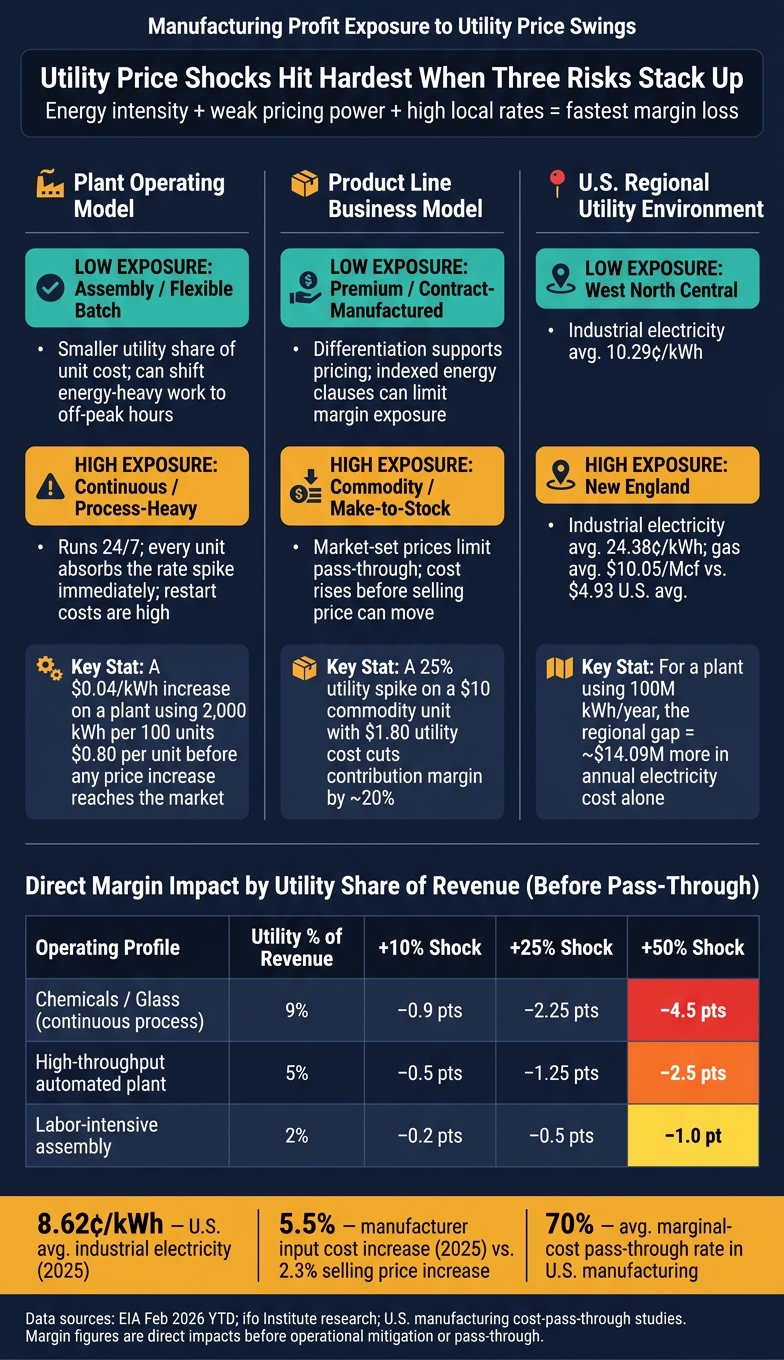
Manufacturing Profit Exposure to Utility Price Swings: Key Risk Factors
| Area | Lower exposure | Higher exposure | Main reason |
|---|---|---|---|
| Plant model | Assembly / flexible batch | Continuous / process-heavy | More energy per unit and less room to shift load |
| Product type | Premium / contracted | Commodity | Less pricing room in market-priced goods |
| Order model | Make-to-order | Make-to-stock | Cost can move before selling price does |
| Region | Lower-rate markets | High-rate markets | Local tariffs, gas spreads, and demand charges |
So if I’m trying to explain profit pressure from utility swings in plain English, the answer is simple: the damage depends on energy intensity, pass-through speed, and local utility cost.
A plant’s operating model shapes how utility price swings show up in profit. Continuous and process plants run equipment 24/7 with steady input and output. One cited model found that a continuous facility could operate 33% more efficiently than a similar batch facility.[2] That edge helps when rates are stable. But when electricity or gas prices jump, the hit lands right away on every unit coming off the line. Restart costs can also be high, and quality can slip if operations are interrupted. The first place this shows up is unit cost. Then it moves into gross margin.
Batch and flexible plants have more room to move. They can shift energy-heavy work into lower-rate hours. That sounds simple on paper, but every changeover brings extra labor, cleaning, downtime, and testing. Customer delivery windows and minimum order sizes can also shrink that room fast, often before any margin relief shows up.
To compare these models, translate plant behavior into utility cost per saleable unit:
$$\text{Utility-cost impact per unit} = \frac{\text{Utility consumption} \times \text{Price change}}{\text{Saleable units}}$$
If a plant uses 2,000 kWh to make 100 units, a $0.04/kWh increase adds $0.80 per unit before any price increase reaches the market.
| Dimension | Continuous | Batch |
|---|---|---|
| Utility cost per unit | Lower at high utilization | Higher with frequent changeovers |
| Exposure to price spike | High - operations continue regardless | Lower - some production can be deferred |
| Ability to reschedule energy-intensive work | Very limited | Moderate, depending on customer constraints |
| Pass-through flexibility | Stronger with indexed contracts | Depends on product differentiation and customer tolerance |
Don’t bury all utility costs inside one overhead bucket. Break out base-load uses like controls, HVAC, pumps, and support systems from consumption tied to production volume. Also track changeover and cleaning energy on their own. Those repeated heating and cooling cycles can quietly make a flexible plant far more utility-intensive than a long production run.
Operating model is the starting point. Product mix decides how much of that shock a business can absorb and how much it can pass through.
Plant cadence tells you when a utility shock shows up. Product-line economics tells you how hard it hits margin.
That split matters. Utility spend often moves with output, but service fees, demand charges, and minimum-take terms can lock in fixed or semi-fixed cost. So two lines in the same plant can feel the same rate jump in very different ways.
Five product-line models tend to react in different ways. The first three are about pricing power. The last two are about repricing speed.
Commodity and highly production-intensive lines usually take the hardest hit. Bulk chemicals, metals, glass, paper, and cement depend on high-temperature heating, refrigeration, drying, pumping, or compressed air. That makes utilities a big part of unit conversion cost. And because prices are usually market-set rather than producer-set, pass-through is limited.
Here’s what that looks like in plain terms: if a commodity product sells for $10.00 per unit and carries $1.80 in utility cost, a 25% jump in utility prices adds $0.45 per unit. That cuts contribution margin by about 20%. On a thin-margin line, that’s a painful squeeze.
Contract-manufactured lines get some cover from customer agreements. Contracts can pass through commodity and energy-price changes, which can limit margin exposure.[4] The catch is in the wording. Good contracts usually spell out:
Premium lines can absorb the same dollar increase with much less damage to percentage margin. Say a product sells for $100.00 per unit, has $3.00 in utility cost, and earns a $45.00 contribution margin. If utility prices rise 25%, contribution margin falls by less than 2%. That’s a much softer blow. The tradeoff is on the demand side: if price hikes come too often, customers may start to pull back.
Pricing power is one side of the story. Order timing is the other.
Make-to-stock producers can get stuck with a lag. They may already be producing at higher utility cost before they can lift finished-goods prices. In that gap, costs go up first and revenue catches up later.
Make-to-order operations can build current utility rates into new quotes, which helps. But they’re not off the hook. Fixed customer commitments and frequent changeovers can still pressure margin while orders are being filled. Short quote-validity windows, escalation clauses, or built-in energy surcharges can help reduce that exposure.
| Product-Line Model | Utility Cost as % of Conversion Cost | Pass-Through Flexibility | Primary Risk |
|---|---|---|---|
| Commodity | High | Low - market-set prices | Margin compression on every unit |
| Contract-manufactured | Moderate | Moderate - depends on contract terms | Fixed-price contracts with no energy clause |
| Premium | Low to moderate | High - differentiation supports pricing | Demand erosion if price increases are too frequent |
| Make-to-stock | Varies | Delayed - inventory timing mismatch | Cost incurred before repricing is possible |
| Make-to-order | Varies | Faster - current rates can enter new quotes | Short lead times and fixed quotes during fulfillment |
These figures are illustrative rather than industry averages. The key insight is that exposure depends on utility cost relative to selling price and contribution margin - not on absolute energy consumption alone.
One more thing: track utility cost by SKU or product family, not just by plant.
A single site might combine low-energy assembly with ovens, dryers, or refrigeration. If you only look at plant averages, weak lines can hide in the mix. SKU-level utility costing makes it easier to spot which lines lose margin first.
And even the same product line can face very different margin pressure from one location to another, depending on local utility rates and tariff structure.
Once the plant model and product mix are locked in, location sets the utility cost floor. Two plants can run the same production profile - 6,000 hours per year, 50 million kWh of electricity, and 500,000 MMBtu of natural gas each year - and still end up with very different utility bills based on where they’re located. That’s why region is the next screen after operating model and product mix.
Even within the same region, market structure changes the picture. ISO-NE in New England, NYISO in New York, SPP in the central states, and ERCOT in Texas don’t move in sync. So regional averages are useful for screening, but they’re not the final answer.
In February 2026 year-to-date data, industrial electricity averaged 24.38¢/kWh in New England versus 10.29¢/kWh in the West North Central region.[5] For a plant using 100 million kWh per year, that difference adds up to about $14.09 million annually in extra electricity cost - before demand charges, tariff design, or hedging even enter the picture.[5] That gap flows straight into unit cost and squeezes contribution margin on every unit produced.
Electricity is only one side of it. Gas spreads can hit just as hard for heat-heavy plants. New England’s industrial gas price is about $10.05 per thousand cubic feet, while the U.S. average is roughly $4.93.[6] Pipeline constraints - not just distance from supply - help explain the gap.[6] For a gas-heavy plant using 1 billion cubic feet each year, that regional difference alone could total $5.12 million annually.[6] That matters most for glass, steel, cement, food processing, and chemical plants, where gas is a major process input.
The same production profile can lead to very different utility costs by region:
| Region | Cost profile | Key utility risk | Best fit |
|---|---|---|---|
| Northeast (New England / Middle Atlantic) | High electricity and gas costs; winter constraints | Fuel constraints and congestion drive spikes | Low-energy, high-margin, or strong pass-through contracts |
| Midwest | Utility-territory differences can outweigh regional averages | Tariff variation within the region | Mixed profiles; model specific utility tariffs |
| South/Gulf Coast | Often favorable on average; spikes from weather and congestion | Load growth and weather events | Gas-intensive and electricity-intensive industrial plants |
| Southwest | Transmission and tariff design drive exposure | Transmission constraints | Flexible loads and sites with pass-through pricing |
| West Coast | High electricity burden; demand charges matter | High effective cost per unit | High-value, differentiated products with pricing power |
| Pacific Northwest | Hydro-backed, but transmission and reliability still matter | Reliability and transmission risk | Electricity-intensive, continuous-process manufacturing |
Texas needs its own model because ERCOT pricing does not track other U.S. markets.
Regional averages also miss tariff-level costs. This is where a lot of people get tripped up. The posted energy rate may look fine, but the billed rate can tell a very different story.
A plant’s effective price per unit can shift based on things like:
Two plants in the same state - even on the same utility - can end up with different effective rates based on voltage level, load factor, and whether they qualify for interruptible or time-of-use tariffs. Those details shape the real cost per unit and, by extension, the margin hit.
Utility price shocks don't hit every plant the same way. The cost mix matters. So does the plant setup, the product mix, and the region's starting utility rate.
Start with the direct effect: apply the utility price change to baseline utility spend, while holding output and non-utility costs constant. For a plant with $10 million in annual revenue and $1.5 million in utility expense, the direct operating profit impact looks like this:
| Utility-price scenario | Change in utility expense | Change in operating profit |
|---|---|---|
| −10% | −$150,000 | +$150,000 |
| +10% | +$150,000 | −$150,000 |
| +25% | +$375,000 | −$375,000 |
| +50% | +$750,000 | −$750,000 |
That gives you the baseline. From there, the comparison comes down to cost intensity, pricing power, and fixed-charge load. Then you layer in mitigation.
Utility share of revenue is one of the biggest drivers of profit pressure. ifo Institute research found that positive electricity-price changes reduce manufacturer profits by about 1.6% on average, with bigger losses for gas-intensive firms.[7] A chemical or glass plant where utilities equal 9% of revenue is in a very different spot from an assembly plant where utilities are only 2% of revenue. In the first case, a +50% shock wipes out about 4.5 percentage points of operating margin before mitigation. In the second, the direct hit is closer to 1 percentage point.
Pass-through flexibility is the other big variable. U.S. manufacturing research puts average marginal-cost pass-through at about 70%, which means firms often recover a large share of energy-driven cost increases through higher output prices, but not all of it.[1] The math is simple:
Net impact = gross utility increase × (1 − pass-through rate).
Under a +50% shock on that $1.5 million utility bill, an 80% pass-through leaves only $150,000 unrecovered. A 30% pass-through leaves $525,000 unrecovered. Commodity producers with market-set prices often land near the low end. Differentiated manufacturers, or firms with energy-adjustment clauses in contracts, can get much closer to the high end. Still, full pass-through protects unit margin at the risk of weaker volume and lower competitiveness.[7]
The same shock can look very different depending on utility share of revenue:
| Operating profile | Utility % of revenue | +10% margin impact | +25% margin impact | +50% margin impact |
|---|---|---|---|---|
| Energy-intensive continuous-process (e.g., chemicals, glass) | 9% | −0.9 pts | −2.25 pts | −4.5 pts |
| High-throughput automated plant | 5% | −0.5 pts | −1.25 pts | −2.5 pts |
| Labor-intensive assembly | 2% | −0.2 pts | −0.5 pts | −1.0 pt |
Figures shown are direct margin-point reductions before pass-through or operational mitigation.
Fixed charges add another layer. Even when pass-through softens the gross shock, the utility bill doesn't move down as much as many operators expect. If $400,000 of a $1.5 million utility bill is fixed or semi-fixed, then a +50% shock on the variable share adds $550,000, not $750,000. But those fixed charges don't go away if output drops. They just get spread over fewer units, which pushes unit utility cost up even if the total bill falls only a little.
At +25% and +50% shock levels, the decision usually narrows to three moves:
Utility shocks hit margins fastest when three things stack up at once: high energy use, weak pricing power, and heavy fixed charges. The table below shows how those trade-offs play out across plant type, product mix, and region. Use it to spot the first point of strain: process rigidity, limited ability to pass through costs, or an expensive operating footprint.
| Operating profile | Margin resilience | Break-even risk | Pricing power | Repricing speed | Grid reliability exposure | Fixed-cost burden |
|---|---|---|---|---|---|---|
| High-energy continuous plant (chemicals, glass, metals) | Low | High | Low–Medium | Slow | High | High |
| Flexible batch plant | Medium–High | Medium | Medium | Medium | Medium | Medium |
| Assembly-heavy facility | Medium–High | Medium | Medium | Medium–Fast | Low–Medium | Medium |
| Commodity product line | Low | High | Low | Slow | Varies by plant | High |
| Premium product line | Medium–High | Medium | High | Medium–Fast | Varies by plant | Medium |
| Contract manufacturing | Medium | Medium–High | Low–Medium | Depends on contract | Varies by plant | Medium–High |
| Low-cost U.S. region | High | Low–Medium | Varies | Varies | Varies | Low–Medium |
| High-cost U.S. region | Low–Medium | High | Varies | Varies | Varies | High |
The pattern is pretty clear. A utility shock turns into margin loss first in continuous plants and commodity product lines. Those setups get squeezed from all sides: they use a lot of energy, they can't pass costs through easily, and fixed charges don't let up when output falls.
Other models have more room to maneuver, but it's not free. Batch plants and assembly-heavy facilities can shift schedules more easily. Premium product lines may have more pricing room. Contract manufacturers may get some help from energy-adjustment clauses. Still, each one gives something up, whether that's speed, margin, or contract flexibility.
One big problem: consolidated financials can blur the real risk. A company-level view might look fine while one plant or one SKU is taking the hit. That's why utility cost should be assigned by driver and tested at the plant and SKU level.
The next move is straightforward: model utility cost by plant and SKU, then run shock scenarios against contribution margin. Phoenix Strategy Group offers fractional CFO, FP&A, and data-engineering services tied to this kind of scenario reporting and plant-by-product margin analysis.
Utility volatility hits hardest when energy makes up a big share of unit cost, production uses a lot of power, and pricing moves on a delay. Those risks get worse in high-cost regions.
The 2025 numbers make that plain: U.S. industrial electricity averaged 8.62 cents per kilowatt-hour, while state averages ran from 8.20 cents in North Dakota to 35.72 cents in Hawaii.[3] At the same time, manufacturers' input costs climbed 5.5% in 2025, while selling prices rose just 2.3%.[8] For energy-intensive plants, that gap can wipe out margins even when the product itself looks sound on paper.
That’s why margin analysis can’t stop at utility rate changes. You need to follow the whole chain from utility cost to cash flow. In practice, that means modeling utility cost per unit, contribution margin, operating income, break-even volume, and cash flow as one connected system.
Use that margin bridge to steer pricing, sourcing, production, and capital decisions. Then turn it into a repeatable model that pulls together utility, production, pricing, and cash data. Phoenix Strategy Group supports this work through fractional CFO, FP&A, data engineering, and strategic advisory services.
Measure energy exposure at the plant and SKU level, not in aggregate.
Sync utility consumption data with production output at the plant or SKU level. Pull actual usage, like electricity, natural gas, or compressed air, from ERP and MES systems. Then use sub-meters or IoT sensors to separate loads by machine or process.
Next, calculate Specific Energy Consumption (SEC) for each SKU by dividing energy used by units produced. That gives you a clear view of how much energy each unit takes to make.
From there, use driver-based models to link those inputs to financial results and track margin impact when utility prices move.
The most exposed models tend to be energy-intensive plants and businesses with high fixed-cost structures. When costs jump all at once, these companies often can't adjust fast enough.
Manufacturers with complex, multi-SKU operations or companies scaling fast face extra pressure too. In those cases, energy use can climb faster than revenue, which puts cash flow in a tight spot.
Utility bills often include two parts: a fixed base charge and usage-based fees. The fixed charge stays the same no matter how much you produce, so it sets a baseline cost even when business slows down.
If utility rates go up, that fixed charge turns into a hard cost floor. And that can squeeze margins even more, because utility expenses don't fall in line with lower output.