Published on
September 4, 2026


A renewable DCF model should answer three things fast: what the asset is worth today, whether the debt works, and how returns change under downside cases.
If I were building or reviewing this model, I’d focus on a short list of drivers first: MWh production, contract price, CapEx timing, OpEx, tax credits, depreciation, debt sizing, and end-of-life costs. In most U.S. renewable deals, a 20- to 30-year forecast, monthly construction periods, and a clean split between project-level cash flows and holdco returns are enough to get to NPV, IRR, DSCR, LLCR, and PLCR.
Here’s the article in plain English:
A quick way to think about it: if your model can’t show base, upside, and downside cases with clean links from assumptions to value, it’s not ready for an investment or lender review.
The rest of the article explains how to build that model step by step.
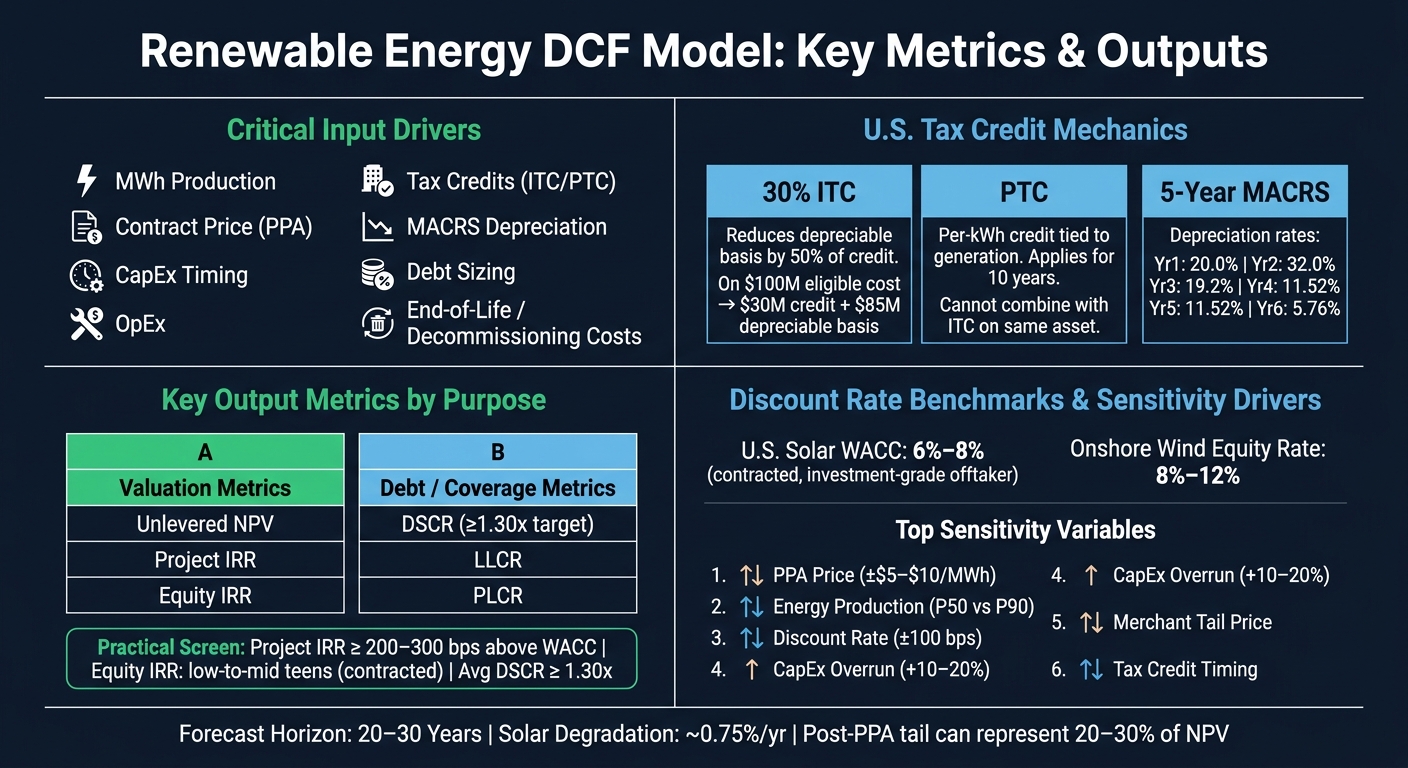
Renewable Energy DCF Model: Key Metrics, Inputs & Outputs Cheat Sheet
Once the valuation question is clear, set up the timeline and model controls first. Build the skeleton before you start dropping in cash flows. In project finance, small structure mistakes can snowball fast.
Set the model end date based on the longest binding obligation. That usually means the PPA term, equipment life, land lease, and interconnection agreement. The model should run through the asset’s full life, with the post-contract period shown on purpose, not skipped over.
When the first PPA ends, keep modeling that period with clear pricing assumptions. That might mean merchant pricing, a renewed PPA, or hedge contracts. Leaving that stretch blank creates a hole right where a lot of value can sit.
If the project includes a mid-life repower, add the related CapEx and any new tax credit eligibility tied to that work. At the end of the asset life, include decommissioning cost. This is often modeled as either a fixed $ amount per MW or a percentage of initial CapEx.
A modular tab layout makes the model easier to audit and easier to scale. It also helps you trace each assumption from the input page all the way to the final outputs. In U.S. project finance, the usual flow is simple: Inputs → Construction → Operations → Tax → Financing → Outputs. Each tab should pull from the tab before it. Nothing should feed back upstream.
| Tab | Primary Purpose | Key Outputs |
|---|---|---|
| Inputs/Assumptions | Single source of truth for all drivers | Capacity (MW), PPA price, CapEx, OpEx, tax rates, financing terms |
| Construction (CapEx) | Time-phased spend from NTP to COD | Periodic cash outflows, cumulative spend, IDC, funding needs |
| Operations | Energy production, revenue, and OpEx | CFADS (Cash Flow Available for Debt Service), unlevered returns |
| Tax & Depreciation | MACRS, ITC/PTC, taxable income, cash taxes | After-tax cash flows, NOLs, deferred tax |
| Financing | Debt, tax equity, distributions, DSCR | Levered cash flows, covenant checks, waterfall |
| Outputs | NPV, IRR, DSCR, scenario summaries | Investment committee–ready metrics |
Use one source of truth for each driver. Don’t hard-code inputs inside formulas. It may feel faster in the moment, but it turns audits and updates into a mess.
The model’s time step should match how the asset earns and spends cash. Use monthly periods through construction and early operations, then move to quarterly or annual periods once the project reaches steady state [7][6]. Monthly detail during construction helps you track milestone-based EPC payments, interconnection draws, and the exact placed-in-service date for ITC/PTC eligibility. For covenant testing, use a separate quarterly debt schedule.
Every model should include three control checks:
If debt sculpting creates circulars, fix them with iterative calculations or an algebraic rewrite.
Once the model structure is set, the next job is simple in theory and messy in practice: put in the numbers. In a renewable energy DCF, cash flow comes from three main buckets: revenue, operating costs, and tax effects.
Start with MWh, not dollars. If the production forecast is weak, the revenue forecast will be weak too.
For solar, model output from year-one MWh and apply 0.75% annual degradation.[14][15] For wind, the bigger swing factor is year-to-year resource variability. So for the base case, use P50 MWh. Then run P75 or P90 cases when testing DSCR and downside risk.
After you have annual MWh, turn that output into revenue by contract bucket. A contracted PPA at $25.00/MWh with 2.0% annual escalation is pretty direct. Merchant revenue is a different story. It moves around more, so it needs a hub price curve plus scenario analysis. One base forecast isn't enough. RECs, capacity payments, and ancillary services should sit in separate lines above energy revenue, since they depend on different drivers than power prices.
Those revenue lines feed operating cash flow, which then rolls into DSCR and valuation.
| Revenue Type | Output Predictability | Price Volatility | Contract Dependence |
|---|---|---|---|
| Solar with long-term PPA | High | Low to moderate | High |
| Wind with long-term PPA | Moderate | Low to moderate | High |
| Solar or wind with merchant exposure | Tech-specific | High | Low to moderate |
Construction CapEx usually includes EPC, interconnection, development, owner's costs, and contingency. The timing matters. So does the label you give each cost, because that affects tax basis and depreciation.
After the project reaches COD, recurring OpEx takes over. For utility-scale solar, O&M often lands around $10–$15/kW per year. Then add land lease payments, insurance, property taxes, and asset management fees. Wind O&M is higher per MW because the equipment is more complex. For escalation, use one steady inflation view across the model. 2.0% to 2.5% per year is common.
Maintenance CapEx is not the same thing as OpEx. That's a line modelers sometimes blur, and it can cause trouble. Solar inverter replacements, often needed every 10 to 15 years, and major wind component work like gearboxes and blades, should show up as one-off capital items in the years they are expected. Don't smooth them across annual OpEx. Those jumps can cut cash available for debt service in a given year, which has a direct effect on DSCR.[1][13]
After revenue and OpEx, move from pre-tax cash flow to after-tax cash flow. This is where ITC, PTC, and MACRS matter. They don't just change total taxes paid. They also change when equity gets its cash flow.
Take a 30% ITC example. The depreciable basis is reduced by 50% of the credit amount. On $100 million of eligible cost, a 30% ITC creates a $30 million credit and leaves an $85 million depreciable basis.[11][12] From there, run the MACRS schedule on that adjusted basis. Qualifying clean-energy property uses 5-year MACRS with half-year convention, which gives depreciation rates of 20.0%, 32.0%, 19.2%, 11.52%, 11.52%, and 5.76% in years one through six.[8][9][10] Because that depreciation is front-loaded, the model gets large early-year tax shields, and that can lift equity IRR even if operating cash flow stays flat.
The PTC works in a different way. It is a per-kWh credit tied to eligible generation, usually for 10 years for qualifying projects. In most cases, you can't claim both ITC and PTC on the same asset, so the model needs a clean election. If the deal uses tax equity, monetization of those credits shifts to the tax equity investor, and that changes both the timing and the size of equity cash flows.
| Cash Flow Item | Category | Model Treatment |
|---|---|---|
| EPC and construction costs | One-time construction CapEx | Pre-tax (sets depreciable basis) |
| Interconnection and owner's costs | One-time construction CapEx | Pre-tax (included in tax basis) |
| O&M, land lease, insurance, property taxes | Recurring OpEx | Pre-tax (reduces taxable income) |
| Inverter replacements, major overhauls | Maintenance CapEx | Pre-tax (depreciated separately) |
| ITC (Investment Tax Credit) | Tax credit | After-tax (reduces tax liability dollar-for-dollar) |
| PTC (Production Tax Credit) | Tax credit | After-tax (reduces tax liability per kWh) |
| MACRS depreciation | Tax shield | After-tax (reduces taxable income) |
| Cash taxes paid | Tax outflow | After-tax (net of credits and depreciation) |
These after-tax cash flows feed the discount rate and terminal value section next.
Once your after-tax cash flows are in place, the next job is turning those cash flows into value. That comes down to two choices: the discount rate and the terminal assumption.
The discount rate needs to fit the cash flow type. If you're discounting unlevered free cash flows, use WACC. If you're discounting levered equity cash flows, use the cost of equity. CAPM is a good place to begin, but it shouldn't be the end of the story. Sanity-check it against what the market is pricing.
For U.S. utility-scale solar with a long-term PPA and an investment-grade offtaker, indicative unlevered WACCs usually land in the 6%–8% range. For onshore wind, equity discount rates often sit in the 8%–12% range.[1][16]
What moves the rate up or down? Usually the same things that shape the operating forecast:
That alignment matters. If the forecast assumes a stable contracted asset, the rate should reflect that. If the model includes merchant tail risk or curtailment pressure, the rate should pick that up too.
A practical way to do this is to start with a contracted-project benchmark, then add 50–150 basis points for non-investment-grade offtakers, construction exposure, or material merchant exposure. The key is to tie those adjustments to market evidence, not gut feel.[18]
The discount rate tells you how hard future cash flows should be hit. Terminal value tells you what the asset is still worth after the explicit forecast period.
For single-asset renewables, the cleanest approach is usually to model the full asset life directly. In plain English, run annual cash flows through the project's technical or contractual life, which is often 25 to 35 years. That lets you reflect degradation, PPA expiries, merchant periods, and end-of-life costs inside the model instead of stuffing them into a shortcut. Even then, the last stretch of the forecast can still account for 20% to 30% of NPV.[17]
Here are the three main approaches and where each fits:
| Method | Best Use Case | Strengths | Limitations in Renewables |
|---|---|---|---|
| Explicit-life DCF | Single-asset project finance, tax equity, lender analysis | Captures degradation, PPA expiry, decommissioning, and repowering decisions; transparent | More complex; assumptions beyond year 15–20 carry increasing uncertainty |
| Gordon growth (perpetuity) | Developer platforms, portfolio valuations with an ongoing project pipeline | Simple to compute; useful for ongoing businesses | Assumes perpetual life, which is a poor fit for finite-life assets; sensitive to small changes in g and r |
| Exit multiple (EV/EBITDA, $/MW) | Sale scenarios and sponsor exits at a defined horizon | Anchored in market pricing; easy to communicate | Sensitive to market cycles; can be misleading if the chosen multiple already reflects optimistic assumptions |
Two pieces often get overlooked: repowering value and decommissioning costs.
For wind, existing interconnection rights can become a major end-of-life asset in constrained markets. In some cases, they can make up 20% to 40% of terminal value.[17] That piece should be modeled on its own, not blended into salvage value.
Decommissioning needs the same treatment. Wind decommissioning can cost tens of thousands of dollars per turbine after salvage, so those cash outflows belong in the final forecast years. If you skip them, the model can paint a much prettier picture than the asset will actually deliver.
Once you’ve set cash flows, discount rate, and terminal value, the model needs to do one thing well: turn those assumptions into financing and M&A calls. And that only works if the earlier inputs - production, costs, taxes, and discount rate - are solid.
A DCF gives you several outputs, but each one answers a different question. Unlevered NPV and project IRR show whether the asset creates value before financing. That makes them the right tools for acquisition screening and internal investment memos. Equity IRR adds the capital structure on top, including debt, tax equity, and distributions to common equity.
For lenders, start with DSCR. Then look at LLCR and PLCR for a longer view of coverage. Those three are financing tests, not valuation outputs.
Put simply, the same forecast should answer three things: value, leverage, and downside resilience.
| Metric | What it tells you | Best used for |
|---|---|---|
| Unlevered NPV | Value created by the asset before financing | Acquisition screening, board review |
| Project IRR | Asset return before debt | Comparing project economics across deals |
| Equity IRR | Return to common equity after debt service | Fundraising, sponsor return discussions |
| DSCR | Ability to cover current-period debt service | Lender sizing, covenant testing |
| LLCR | Coverage over the remaining loan life | Longer-term lender comfort |
| PLCR | Coverage over the full project life | Ultimate project solvency assessment |
A practical U.S. committee screen is project IRR at least 200–300 bps above WACC, equity IRR in the low-to-mid teens for contracted assets, and average DSCR ≥ 1.30x.
After you review the core outputs, test the assumptions that matter most. Not every input needs its own sensitivity tab. The goal is to focus on the variables that move NPV and IRR in a meaningful way.
For contracted projects, the biggest drivers are usually price and production. For merchant-heavy assets, the pressure points are power curves and discount rate. A 5%–10% change in net energy yield can shift unlevered IRR by 50–150 basis points and can also tighten DSCR and LLCR. A ±100 basis point move in discount rate, or even a modest change in merchant price assumptions, can move IRR by several percentage points when much of the value sits in an uncontracted tail.
Here are the main sensitivities by asset type:
| Sensitivity Variable | Direction of Impact | Most Material For |
|---|---|---|
| PPA price (±$5–$10/MWh) | Higher price → higher NPV and IRR | Contracted assets |
| Energy production (P50 vs. P90) | Lower production → lower NPV, IRR, DSCR | Both; critical for debt sizing |
| Curtailment (2%–5% reduction) | Higher curtailment → lower NPV and DSCR | Merchant-heavy and constrained-grid assets |
| CapEx overrun (+10%–20%) | Higher CapEx → lower IRR, higher equity check | Both; especially development-stage projects |
| OpEx inflation (3%–5% vs. 2%) | Higher OpEx → erodes equity cash flow over time | Both; compounds over long asset lives |
| Tax credit treatment | Loss or delay of ITC/PTC → significant NPV reduction | Contracted assets with tax equity structures |
| Merchant tail price | Lower prices → lower NPV and PLCR | Merchant-heavy and post-PPA assets |
| Discount rate (±100 bps) | Higher rate → lower NPV; more visible in long-dated cash flows | Both; especially merchant-heavy assets |
Use P50 as the base case, then stress it with P90 or another downside production case for lender talks and debt sizing. For board and investor materials, a simple scenario view - base, upside, and downside - with equity IRR and NPV side by side is much more useful than a dense formula audit.
A renewable DCF should be simple, accurate, and easy to audit. When production, contracts, costs, taxes, and end-of-life assumptions roll into one clear value case, the model can produce a defendable NPV, IRR, and financing view.
ITC, PTC, MACRS, and tax equity need to sit in the base model because they change timing, not just total value. That matters. These items shape after-tax equity cash flows and deal structure starting in year one of operations. After that, the next question is straightforward: are those cash flows being discounted at the right risk rate?
Use a project-specific discount rate. Contracted operating assets should carry lower discount rates than merchant development assets. Then comes the stress test.
Scenario analysis is the last check. If value falls apart under modest downside cases, the model is not ready for diligence. That is the minimum viable DCF: simple, traceable, and ready for a decision.
Phoenix Strategy Group supports renewable-energy teams with financial modeling and M&A advisory for funding and exit decisions.
It depends on your project’s financial setup and how the asset makes money. ITC is a one-time credit tied to eligible project costs. PTC is a recurring credit tied to the electricity the project produces over a set period.
In your DCF, match the credit to the way the deal is financed and to your tax equity structure. In some cases, the economics may point to both, where allowed. But check the tax rules first, along with transferability rules for your asset type.
Use a monthly model when you need to track variables that shift during the year, such as seasonal production, merchant price forecasts, or specific revenue trends.
It also matters when you’re reconciling generation against technical performance reports, especially when those reports include 12 to 24 months of operating data. The same goes for monitoring cash flows like debt service, operating expenses, and contract-specific volume caps.
Segment cash flows by risk profile.
Merchant cash flows carry more risk than the fixed-price PPA period. They face market price swings, price cannibalization, and basis risk. Because of that, they usually warrant a higher discount rate, often 9% to 14%.
Use conservative long-term price assumptions instead of current spot or forward prices. Also account for decommissioning, repowering, and re-permitting risk.
To estimate a value range, run sensitivities on: