Published on
August 26, 2026


A solar asset can look overpriced or underpriced just because a model handles the PPA the wrong way. In most cases, value moves on five inputs: price, escalator, term, credit risk, and curtailment/volume rules.
If I were reviewing this kind of valuation, I’d check these points first:
The short version: I would not accept a headline valuation until I traced each of those inputs back to the signed PPA, the production report, and the market assumptions in the DCF.
This article explains where those adjustments sit in the model and what I’d review line by line before relying on the number.
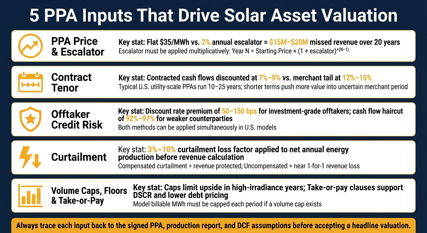
5 PPA Inputs That Drive Solar Asset Valuation
The revenue tab turns PPA terms into forecast cash flow. And this is one of those places where a small input mistake can snowball through the DCF.
Annual revenue is simple on paper: delivered MWh × PPA price.
The tricky part is the escalator.
Many U.S. solar PPAs include a yearly price increase, such as 2% per year or CPI-linked indexation. That increase should be applied multiplicatively, not additively.[1][2][3] The formula is:
Year N price = starting price × (1 + escalator)^(N−1).
That math has a big effect over a 10- to 20-year contract. Say a project delivers 100,000 MWh per year. If an advisor keeps the price flat at $35/MWh instead of applying a 2% annual escalator, the model understates nominal contracted revenue by about $15 million to $20 million over a 20-year term. Even after discounting at standard equity hurdle rates, that can still mean a multi-million-dollar change in NPV.
In plain English: small escalator mistakes can turn into large valuation mistakes.
After the price is set, check that the contract runs through the right end date.
The PPA tenor decides how many years get lower-risk treatment in the model. It also marks the point where the model moves from contracted cash flow to merchant pricing.
In the U.S., utility-scale and corporate PPAs often run 10 to 25 years, with many landing in the 15- to 20-year range. Some newer contracts have shortened to 7 to 15 years.[4]
When the PPA is shorter, more of the asset's value gets pushed into the merchant tail. That's where price uncertainty becomes a bigger issue, and investors tend to apply steeper haircuts. So don't just glance at the contract term. Make sure the model uses the full signed tenor and clearly shows the year when merchant pricing starts.
Review the revenue schedule year by year. Focus on these items:
| Item to Check | What to Look For |
|---|---|
| Stated PPA price | Exact $/MWh from the signed contract |
| Escalation rate and mechanism | Annual percentage or index matching contract language exactly, including any caps, floors, or step changes |
| Commercial operation date (COD) | Model should not start PPA revenue before COD; check for any stub period in the first year |
| Annual delivered MWh | Compare modeled production against engineering estimates and the PPA's contracted volume structure |
| First and final contract year | Confirm the full tenor is used |
| Contracted vs. merchant labeling | Each year should be clearly flagged as PPA or merchant in the revenue tab |
Two mistakes tend to cause outsized damage:
Either one can throw off valuation by tens of millions of dollars in nominal revenue before discounting. It's worth asking the advisor to walk through the revenue tab line by line against the executed PPA.
After the revenue path is set, the next big valuation swing comes from credit risk, curtailment, and volume constraints.
After price and tenor, solar value tends to move most because of credit risk, curtailment, and volume limits. In practice, these three inputs drive most of the next round of valuation changes.
Offtaker credit risk usually shows up in a DCF in one of two ways: a discount-rate premium or a cash-flow haircut.
For investment-grade offtakers, analysts often add 50–150 basis points to the discount rate used for PPA cash flows. For weaker or unrated counterparties, many teams would rather use a direct cash flow haircut instead. That usually means modeling only 92–97% of billed revenue as collectible, then layering in downside cases for partial or full default.
In the U.S., it’s common to use both methods at once: a moderate premium on contracted cash flows, plus separate downside cases with haircuts linked to expected default probabilities and recovery rates.
When you review the model, get specific:
Curtailment should be modeled before revenue. Start with gross generation, subtract curtailment, and then apply volume limits to arrive at billable MWh. Analysts usually apply a curtailment loss factor of 3–10% of net annual energy production before calculating PPA revenue and any REC sales.
The big split here is compensated vs. uncompensated curtailment.
With compensated curtailment, the offtaker pays as if the energy had been delivered. So even if physical output is lost, revenue may not fall by the same amount. With uncompensated curtailment, each point of lost generation is close to a one-for-one hit to revenue. That changes project value fast.
Founders should check how the model handles this. Is curtailment treated as a cut to MWh, a cut to revenue, or both? And does the model match the PPA language on grid curtailment vs. economic curtailment? A small modeling miss here can throw off the whole picture.
Caps, floors, and take-or-pay clauses change both revenue certainty and DSCR.
Volume caps limit the number of MWh the offtaker has to buy, no matter how much the plant produces. Billable MWh need to be capped in each period. Any extra output may earn merchant pricing, or nothing at all. If the cap is modeled the wrong way, PPA revenue can look higher than it should, and lender DSCR can get distorted - especially during strong solar production periods.
Floors and take-or-pay clauses work in the other direction. They help protect revenue.
A volume floor guarantees payment for a minimum annual MWh amount. A take-or-pay clause requires the offtaker to pay for a fixed amount whether delivery happens or not, subject to stated exclusions. That lowers volatility and supports DSCR. It can also help with leverage or debt pricing.
| PPA Structure | Volume Treatment | Curtailment Treatment | Revenue Stability | DSCR Impact |
|---|---|---|---|---|
| Energy-only, no caps | All net delivered MWh billed | Often uncompensated for economic curtailment | Moderate; tracks generation and curtailment | Moderate; sensitive to irradiance and curtailment assumptions |
| Annual/hourly volume cap | Billable MWh clipped at cap; surplus may be merchant or unpriced | Typically uncompensated; some contracts limit curtailment frequency | Lower in high-output periods; constrained upside | More volatile; DSCR suffers when generation exceeds contractual volume |
| Volume floor (minimum take) | Guaranteed minimum billable MWh per year | Curtailment may not reduce payments up to floor if protected | Higher; downside revenue protected | Higher and more stable; improves on guaranteed minimum cash flows |
| Take-or-pay | Fixed payment stream regardless of actual offtake (subject to exceptions) | Often compensated up to contractual obligation | Very high; largely fixed revenue | Very high; supports greater leverage and lower debt pricing |
| Compensated curtailment PPA | May be capped or uncapped; key feature is payment for certain curtailed MWh | System and some economic curtailment compensated at PPA price within defined limits | Higher than uncompensated structures | Higher; DSCR less sensitive to curtailment forecasts |
A simple way to size the value of these protections is to compare DSCR with and without floors or take-or-pay terms.
These are the assumptions founders should test line by line in the model review below.
Use the contract terms above as a line-by-line check on the model. The safest way to review a solar asset valuation is to break the model into three buckets: revenue assumptions, operating and production assumptions, and risk assumptions. Then trace each major input back to the signed PPA, the engineer's production report, or a market source.
Start with the revenue tab. Put the signed PPA next to the model and confirm that the price, escalator, contract dates, and volume terms match the contract language exactly. If the model says one thing and the signed PPA says another, flag it right away.
Then move to the production tab and compare it against the technical report. Make sure the generation inputs line up with the engineer's report. After that, check the risk inputs: the discount rate, credit spread, merchant deck, and curtailment rate. Each one should tie back to a market source or credit analysis, not sit in the model as a mystery adjustment.
Once the base case lines up with the source documents, test the inputs that change NPV the most.
Run one-variable sensitivities on:
These tests show which PPA terms actually change enterprise value. Discount rate and tenor usually move NPV the most because they drive the merchant tail. That output makes it clear which terms you should negotiate first. Ask your advisor for a ranked sensitivity output before any board or investor discussion.
If you're dealing with layered PPA structures, bring in a modeling specialist to audit the formulas before board or lender review. This is one of those areas where a small formula error can snowball.
If the model includes complex PPAs with layered escalators, curtailment compensation, or hybrid merchant revenue, one mis-modeled take-or-pay clause or degradation assumption can move NPV by millions. If the model includes layered escalators, curtailment compensation, or hybrid merchant exposure, have Phoenix Strategy Group audit the formulas before you rely on the valuation.
Put simply, these terms decide how much of a solar project is contracted and how much is left merchant. And in most models, five PPA terms drive most of the movement in solar DCF value.
PPA price and escalators shape the revenue line for every contracted year. Even a $2–$5/MWh gap can snowball over a 15- to 25-year contract and lead to a big swing in equity value. Contract tenor matters just as much. It sets how long those contracted cash flows stay in place before the model moves into the merchant tail, where cash flows face a higher discount rate and more price uncertainty.
Offtaker credit risk hits the model from two angles. It can push up the discount rate, or it can show up as a haircut to expected collections. A weaker counterparty increases the discount rate premium and cuts debt capacity. That, in turn, changes how much equity the deal needs.
Curtailment and volume limits are easy to overlook, but they matter a lot. Lenders apply curtailment haircuts straight to modeled annual MWh, which lowers revenue and debt capacity by roughly the same share.[5] Volume caps can limit upside in high-irradiance years, while take-or-pay clauses help support contracted cash flow.
The main takeaway is simple: test the inputs, not just the headline value. Review the DCF line by line against the signed PPA. Then run sensitivities on:
A single mis-modeled curtailment clause, or a default escalator that doesn't match the signed PPA, can shift NPV by millions without being obvious in the summary output. Traceable inputs help cut surprises and make financing discussions cleaner.
If the structure is complex, Phoenix Strategy Group can audit DCF models, tie PPA contract language to financial inputs, and run sensitivities that show which terms move value the most.
The PPA term sets how long a project’s cash flow stays locked in and under contract before it moves into merchant-tail exposure. If that term is short, more of the valuation depends on market forecasts. It also makes the model more sensitive to assumptions about the merchant period.
In a DCF, analysts split those revenue phases apart. They usually apply a lower discount rate during the fixed-price PPA term and a higher rate to the merchant tail. The result is a blended valuation that reflects how the project’s risk changes over time.
Usually, it’s both. It depends on the counterparty and the level of risk involved.
Investment-grade utilities and highly rated corporate buyers may support a lower discount rate. Their payment risk is often lower, so using the same rate across every revenue stream can blur the picture.
Weaker counterparties often call for direct cash flow adjustments instead. That can mean probability-weighted default assumptions or higher credit-loss reserves. Don’t use one blended rate for everything. Use tiered discount rates that match the credit quality and risk profile of each revenue stream.
In a discounted cash flow model, curtailment and volume caps are built straight into projected energy output and revenue.
Curtailment cuts expected generation in MWh based on congestion patterns or ISO-level scenarios, not on the plant’s maximum theoretical output. That matters because a project may be able to produce more on paper than the grid can actually take in practice.
Volume caps work on the revenue side. They limit revenue to the contracted quantities at the agreed prices, even if the project produces more energy than the contract covers.
These adjustments are made at the project level and then stress-tested through sensitivities to show downside cash flow risk.