Published on
July 23, 2026


A solar portfolio is not just one project multiplied by ten. Once I move from a single asset to a fleet, value changes because risk, contract mix, geography, asset age, and shared costs all change the cash flow picture.
Here’s the short answer:
A few numbers frame the issue:
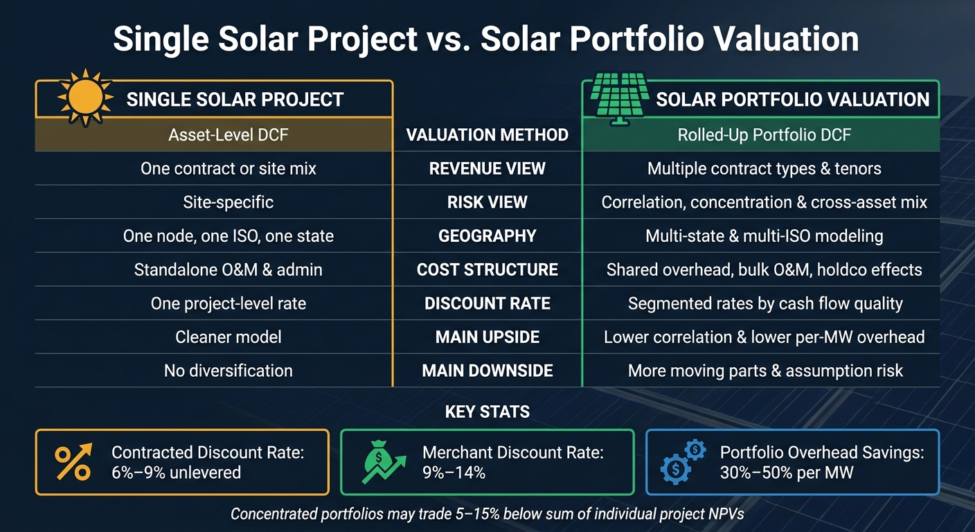
Single Solar Project vs. Portfolio Valuation: Key Differences
| Area | Single Solar Project | Solar Portfolio |
|---|---|---|
| Main valuation method | Asset-level DCF | Rolled-up portfolio DCF |
| Revenue view | One contract or one site mix | Multiple contract types and tenors |
| Risk view | Site-specific | Correlation, concentration, and cross-asset mix |
| Geography | One node, one ISO, one state setup | Multi-state and multi-ISO modeling |
| Cost structure | Standalone O&M and admin | Shared overhead, bulk O&M, holdco effects |
| Discount rate | One project-level rate or contracted/merchant split | Segmented rates by cash flow quality |
| Main upside | Cleaner model | Lower correlation and lower per-MW overhead |
| Main downside | No diversification | More moving parts and more assumption risk |
My takeaway: if you’re valuing a single project, a clean project DCF usually does the job. If you’re valuing a fleet, the hard part is not the math. It’s making sure the model reflects how the assets behave together, not just what each asset does on its own.
A single solar project is usually valued with an after-tax DCF model. The model projects cash flows over 25 to 35 years and discounts them back to today using a project-specific discount rate. That gives you the base case before portfolio effects change the picture.
Start with annual MWh production. Then apply availability and annual degradation assumptions, usually 0.3% to 0.7% per year. From there, price the output using the PPA rate or the merchant curve, then subtract O&M, lease payments, insurance, taxes, management fees, and reserves.[2]
What’s left is net cash flow to equity. In the early years, ITC and 5-year MACRS push more value upfront, which can have a big effect on present value.[4]
Single-asset contracts are often pretty simple: one PPA, one counterparty, one pricing profile.
The cleanest case to model is a fully contracted project with a 15- to 25-year fixed-price PPA and an investment-grade utility offtaker. In that setup, revenue is basically price × MWh, adjusted for any escalation schedule, and risk stays fairly contained.[1]
A merchant tail is different. It needs its own pricing view and its own discount assumptions for the uncontracted years. Even for one project, it’s standard to treat contracted cash flows and merchant cash flows as carrying different levels of risk.
Once the contract structure is locked in, location becomes the next big driver of project-level risk.
A single project carries concentrated production and pricing risk at one site. There’s no portfolio effect to smooth out weak output or soft pricing somewhere else.
Irradiance and temperature at the site drive the capacity factor assumption. Interconnection terms and nodal congestion patterns also matter because they affect realized prices and curtailment risk.[6]
Technology choice matters too. Single-axis tracking usually lifts annual yield versus fixed-tilt, but it also adds O&M complexity. So both the production gain and the added cost need to show up in the model. Sensitivity work should test production, basis, and curtailment risk.
The discount rate should match the asset’s risk profile.
For contracted utility-scale solar with an investment-grade offtaker, unlevered discount rates in the U.S. usually fall in the 6% to 9% range. Rates tend to sit closer to 6% to 7% for long-term PPAs with rated utilities, and closer to 8% to 9% for shorter contracts or weaker counterparties.[1]
In practice, investors anchor that rate to comparable transactions and current financing terms, with CAPM used as a reference input.
At portfolio scale, those same inputs get blended across assets, and that changes both cash flow volatility and the discount rate.
Portfolio valuation starts with one simple move: put every project on the same financial footing, then roll those cash flows into a single forecast. The valuation framework itself doesn't change. What changes is how risk gets mixed across assets and how that blended risk gets priced.
At the portfolio level, the big shift isn't the DCF method. It's the way assumptions are standardized and rolled up across assets.
That means using the same forecast horizon across the portfolio, the same inflation view, production forecasts in MWh, and contract revenue assumptions in U.S. dollars with matching escalator logic.[2][8]
Once those inputs are aligned, revenue, EBITDA, and free cash flow can be rolled up to the portfolio level. From there, portfolio-level adjustments come into play.
Some of those adjustments are pretty practical. Centralized asset management, monitoring, and reporting can cut per-project G&A. Shared spare parts and bulk O&M contracts can also bring down per-project costs. For utility-scale solar, O&M often runs about $8 to $15 per kW-year.[1][8] Portfolio financing can help too, since a larger and more diversified collateral pool may lower rates or extend tenor.[5][3]
Each revenue stream should be discounted based on its contract type. Not all megawatt-hours are worth the same.
Long-term PPAs with investment-grade utilities usually support the lowest discount rates. Shorter C&I contracts, unrated offtakers, and merchant exposure carry more risk. At the portfolio level, the usual approach is to discount each stream based on contract quality, tenor, and offtaker credit, then add up the present values. Investors also watch weighted-average contract tenor and offtaker credit quality closely because both say a lot about cash flow quality.[1][8]
Revenue quality and geographic spread work together here. They shape how much cash flow correlation is still left in the portfolio.
Spreading assets across multiple states and ISOs like CAISO, ERCOT, and PJM can reduce correlation in both output and pricing. That's a big deal. If one region has a rough year, the whole portfolio doesn't have to sink with it if other markets hold up.[8]
Asset age matters too. Seasoned assets with a stable operating history usually support tighter production and downtime assumptions than newer projects. Put those factors together, and lower correlation can support slightly lower discount rates than a similar single-site exposure.[5]
The catch is that the model gets harder to build. Each asset needs local assumptions for curtailment, congestion, basis risk, tariff structures, interconnection rules, and tax treatment.[3][8]
That lower correlation is the main reason portfolio-level discount-rate adjustments can make sense.
At the portfolio level, the discount rate should reflect the combined risk of contract mix, geography, asset age, and concentration. It's not just a simple average of project-by-project rates.
Portfolios built around seasoned, contracted assets with investment-grade offtakers can support unlevered discount rates in the 6% to 9% range. Portfolios with heavy merchant exposure, earlier-stage assets, or concentration in a single ISO can move into the low double digits.[1][5][7][9]
Portfolio scale doesn’t change the core methods. It changes the inputs and how risk gets handled. You see that most clearly in cash-flow rollups, comp selection, and discount-rate blending.
A portfolio DCF adds another layer before you get to one combined value. Each asset still needs its own model, built from asset-level operating facts and policy assumptions. From there, those models get rolled into one forecast, with shared overhead spread across projects, including centralized O&M, asset management, and corporate G&A.
The discount-rate logic changes too. Instead of using one rate across the board, analysts usually apply tiered rates based on contract quality. Long-term investment-grade PPAs often fall in the 6–9% unlevered range, while merchant tail cash flows can land closer to 9–14%. Those rates then feed into a blended portfolio discount rate.[1]
That rollup effect also changes how buyers look at deal comps.
At portfolio scale, the comp set moves away from one-off project sales and toward platform and portfolio deals. Buyers may pay higher multiples when a portfolio has broad geographic spread, a large share of long-dated contracted revenue, and lower financing costs.
The flip side is just as important. Heavy merchant exposure, contract concentration, or operational complexity can push multiples down compared with single-project marks.[10][1][7]
In practice, analysts don’t just pull one EV/MW multiple and call it a day. They usually adjust observed figures for:
At that stage, replacement cost acts more like a floor than the main answer.
For an operating portfolio with contracted cash flows already in place, replacement cost matters much less. It misses things that can drive value in a live portfolio, like above-market PPAs, favorable interconnection rights, and the diversification built into the asset mix over time.
That’s why practitioners usually treat replacement cost as a floor or a reasonableness check, not the lead valuation method.[11][12][13]
The table below boils down the shift from single-asset work to portfolio-scale valuation.
| Approach | Single-Asset Focus | Portfolio-Scale Shift | Primary Limitation at Scale |
|---|---|---|---|
| Income (DCF) | One contract, one rate | Asset rollups, shared overhead, tiered rates | Requires standardized inputs across all assets |
| Market (Comparables) | Single-project deal comps | Platform and portfolio comps; adjusted for contract mix and geography | Requires normalization for contract quality and leverage |
| Cost (Replacement) | $/W installed near COD | Aggregated EPC costs; economies of scale may reduce per-watt cost | Doesn't reflect contracted cash flow value or synergies |
After asset-level cash flows are rolled up, portfolio value comes down to three things: correlation, shared costs, and concentration.
Portfolio models should use correlation instead of simple summation. Why? Because risk only drops when assets aren't moving in lockstep. If you just add projects together, you end up assuming perfect correlation across assets, which makes portfolio risk look worse than it is.
Research across more than 400 renewable projects found that modeling correlation the right way led to a 4.2% improvement in portfolio-wide P95 revenue. For solar-only portfolios, the gain was smaller - about 0.9% - because solar irradiance is often more closely linked across nearby sites.[14]
Regional spread matters too. Assets in different regions or ISOs can have different seasonal patterns, and that can smooth revenue swings. In plain English: one project's softer period can be offset by another project's stronger one. That kind of balance can support a lower discount rate.
Curtailment and settlement timing also change at the portfolio level. Instead of using the same flat assumption for each project, analysts can model ISO-level curtailment cases that hit several assets at once. That gives a more realistic view of downside risk.
The same basic logic applies to operating costs as well.
Scale can trim per-MW overhead by 30–50%, and that can push portfolio value higher when the savings hold up over time. In one real-world analysis of four renewable portfolios, scale synergies and geographic clustering increased total portfolio value by 9.4% and lifted nominal IRR from about 20.3% to 22.3% per year.[16]
That math is pretty simple: lower operating costs mean more free cash flow. And when operations are easier to manage and forecast, buyers may accept a tighter discount rate.
But this isn't automatic. Shared overhead can go sideways if the portfolio grows faster than the team and systems behind it. When that happens, compliance can slip, reporting gets muddy, and investors may apply a valuation discount for governance risk instead of paying up for efficiency.
So cost savings only help if they don't create a new problem somewhere else - especially concentration risk.
A portfolio can look diversified at first glance and still be exposed in a big way. If most revenue comes from one ISO and one utility offtaker, the whole setup may still hinge on the same set of risks. Portfolio modeling tends to make that visible fast.
In concentrated portfolios, buyers may price assets 5–15% below the simple sum of individual project NPVs.[15][17]
Here's where aggregation tends to help - and where it can hurt:
| Factor | Aggregation Premium | Aggregation Discount |
|---|---|---|
| Off-taker mix | Multiple creditworthy counterparties | Single dominant utility (80–90%+ of revenue) |
| Geography | Multiple states and ISOs | Concentrated in one state or congested ISO |
| Production correlation | Low correlation across sites | High correlation (same node, same irradiance zone) |
| Overhead structure | Centralized, scalable, well-documented | Under-resourced or opaque central team |
Those valuation effects get stronger once contract mix enters the model.
At the portfolio level, contract mix matters just as much as production and geography. The way a solar contract is set up drives asset value because it shapes price certainty, counterparty risk, and contract term. You can often value a single project from one contract profile. A portfolio is different. Once several contract structures sit side by side, the picture gets more complicated.
A single long-term PPA is simpler to value. You have one price path, one counterparty, and one main set of assumptions. The cash-flow model is easier to build, and the risk view stays more uniform through the contract period.
The downside is concentration. The asset depends on one off-taker. If that counterparty’s credit starts to weaken, or if the contract offers limited curtailment protection or no negative-price floor, value can drop fast, even if the term is long.
That simplicity fades once a portfolio starts mixing contract types.
Most portfolios include more than one contract type. That means each revenue stream should be modeled on its own. A single blended discount rate can blur major risk differences.
A realistic portfolio might include a utility-scale project under a fixed-price PPA, a community solar asset with subscription revenue and churn risk, a project under a virtual PPA, and a merchant asset tied to spot markets. The practical move is to segment revenue by contract type and risk, apply separate discount rates, and then combine the present values. Long-term contracted cash flows usually support lower rates. Merchant tail cash flows need higher rates. At scale, that spread can change value by a lot.
Model each revenue tranche on its own, then combine present values.
| Revenue Type | How It's Modeled | Key Risk | Discounting Approach |
|---|---|---|---|
| Fixed-price PPA | Contracted payments at agreed price and term | Off-taker credit, curtailment, production underperformance | Lower discount rate for investment-grade, long-duration contracts |
| Virtual PPA | Cash settlement against a hub price and strike | Basis risk, settlement mechanics, credit support | Discounted separately from physical PPA cash flows [18][19] |
| Community solar subscription | Subscriber-based recurring revenue | Churn, payment reliability, program rules | Higher risk adjustment for revenue durability |
| Hedge / contract for differences | Price differential settlement on specified volume | Price forecast error, basis, hedge ratio mismatch | Segmented into hedge revenue and exposed revenue |
| Merchant exposure | Forward curves or long-term price forecasts | Price volatility, basis, no contractual floor | Highest discount rate; widest sensitivity ranges |
Revenue quality comes down to collectability, not just price. Off-taker credit quality should shape both the default adjustment and the discount rate. Investment-grade utilities and highly rated corporate buyers usually support lower credit-loss reserves and lower required returns. Weaker counterparties may call for probability-weighted default adjustments or higher reserves built straight into the model.
Remaining contract term also changes the value picture. Longer terms lock in more value, cut forecast uncertainty, and usually support lower discount rates. Shorter remaining terms push more value into post-expiration merchant assumptions, which makes the asset more sensitive to power prices and re-contracting results.
In a portfolio with staggered expirations, that creates a ladder of re-pricing events. Staggered expirations spread repricing risk. Clumped expirations stack that risk into the same period. Escalation clauses and settlement mechanics add one more twist. A contract that settles financially against a hub index, instead of physically at the plant node, brings in basis risk that can trim the value of contracted cash flow.
Contract mix sets the revenue base; location and asset age determine how stable that base is.
Where a solar project sits - and how long it has been running - can matter just as much as the contract behind it. At portfolio scale, location and asset age shape both forecast cash flow and the discount rate.
A single-site project puts a lot of weight on one ISO, one utility, and one rule book. If that state changes policy or congestion builds at that node, the whole project feels it.
A multi-ISO portfolio is different. Each market needs its own model because pricing, congestion, and curtailment vary by ISO. Regional PPA prices can differ a lot, so portfolio models should use market-specific price curves instead of one blended assumption.
That leads to a simple but important point: multi-ISO portfolios need segmented cash-flow models by market. A single blended forecast won't do the job. Each sub-portfolio should carry its own price curve, curtailment assumption, and state-level policy risk overlay.
| Factor | Single Site | Multi-State Portfolio |
|---|---|---|
| State policy exposure | Concentrated in one regime | Spread across multiple RPS and incentive structures |
| ISO/market design | One ISO, utility, and rule set | CAISO, ERCOT, PJM, MISO, and NYISO modeled separately |
| PPA pricing | Reflects one regional market | Modeled with market-specific price curves |
| Curtailment risk | Concentrated at one node | Spread across regions, with systemic risk within each ISO |
| Modeling complexity | Lower | Higher; requires segmented cash flows and risk overlays |
That market split leads straight to the next issue: how much operating history the assets actually have.
New-build assets are priced off modeled assumptions - engineering energy estimates, equipment warranties, and loss factors. That leaves real uncertainty around commissioning and early performance.
Older assets change that picture. Actual SCADA data, historical availability records, and observed degradation start to replace modeled guesses. So older assets should be valued on observed performance and remaining life, not only on long-run modeled output.
The catch is near-term capex risk. Inverters usually have expected lifetimes of 10–15 years, so a project commissioned in 2012 or 2013 may already be close to inverter replacement. Modules degrade at about 0.5%–0.7% per year, and that compounds over a 20- or 25-year project life.
In a mixed-age portfolio, younger assets tend to bring long-dated contracted cash flows with lower near-term maintenance needs. Older assets bring observable performance, but they also come with shorter remaining contract life and near-term capex.
That split should show up in the valuation method. In practice, that often means tiered discount rates or segmented cash-flow blocks - one for the contracted period and another for post-contract merchant exposure. Asset age should also shape the re-contracting probability and the expected terms.
Once age is set, weather, basis, and curtailment decide how much of that revenue actually shows up.
A broader geographic footprint can reduce production volatility. Solar irradiance correlations drop fast with distance, and research shows monthly production correlations fall steeply up to roughly 1,500 km.[20]
Basis risk is the tougher piece. In organized markets, the gap between a project's settlement node and the reference hub can be large, and it does not behave the same way across ISOs. If a portfolio valuation uses hub-level price forecasts without adjusting each node for basis, it will overstate realized revenue.
The better approach is to build separate basis curves by node or cluster, using historical spreads and scenario analysis for planned transmission additions. From there, basis-adjusted revenues can be aggregated at the portfolio level.
Geography, asset age, and contract mix feed straight into the discount rate. That rate is just a way of pricing risk and a buyer’s comfort level with uncertainty. But once you move from a single project to a portfolio, those same inputs don’t land the same way.
For individual projects, operating assets with long-term PPAs usually sit at the low end of the range. By contrast, development-stage assets or assets with heavy merchant exposure tend to sit higher.
Stage matters because it changes the return buyers expect. Capital structure matters too, since the debt-and-equity mix shapes the blended WACC.
At the portfolio level, the rate shifts because project risks are grouped together. Diversification reduces the odds that one asset will make or break the outcome, so a set of similar operating assets can often support a lower rate.
Larger portfolios can also draw institutional capital more easily. They may offer better exit liquidity as well, which can push required returns down.
Mixed portfolios need a split approach. Operating cash flows should use one rate, while development cash flows should use a higher one.
The table below shows how diversification, concentration, and liquidity turn into actual rate outcomes.
| Scenario | Rate vs. Single-Asset Rate | Why |
|---|---|---|
| Diversified, multi-asset, all operational | Lower | Reduced single-asset risk; better exit liquidity |
| Large portfolio with high debt leverage | Lower (WACC) | Higher debt mix can lower the blended WACC |
| Mixed lifecycle (operational + development assets) | Higher (segmented) | Development cash flows require a separate, higher rate |
| Concentrated geography or single off-taker | Higher | Less diversification increases risk |
| Illiquid or complex structure | Higher | Lower exit liquidity raises required returns |
Those differences shape how investors underwrite the portfolio and what they’re willing to pay for it.
At the portfolio level, the core question is pretty simple: how much asset-level detail does the deal need, and how much roll-up efficiency can the buyer actually use?
That balance shapes the right valuation method. Some approaches work best for a single project with clean inputs. Others make more sense when a buyer is looking at a scaled platform and wants to price in diversification, shared costs, and operating leverage.
Use this grid to line up the valuation method with deal complexity, data quality, and buyer expectations.
| Framework | Pros | Cons |
|---|---|---|
| Single-asset DCF | Clean model; clear attribution to one site and contract set | No diversification effect; no scale benefit |
| Portfolio DCF | Captures diversification, shared costs, and scale; supports platform pricing | Assumption-heavy; requires harmonized inputs; slower to underwrite |
| Market multiples | Familiar to buyers; project comps for simple assets, platform comps for scaled portfolios | Less granular; sensitive to comp selection; misses contract quality and geography differences |
| Replacement cost | Useful floor or sanity check | Doesn't reflect contracted cash flow value |
The same factors that shape valuation also shape buyer demand: contract quality, geography, and operating history. Put bluntly, buyers pay more for predictable contracted cash flow, strong offtaker credit, and a clean operating record.
Operating portfolios with long-term PPAs have traded at $1.0 million to $1.8 million per MWac, with value tied to PPA quality, remaining term, geography, capacity factor, and age.[1]
Buyers running an acquisition-led platform strategy tend to view things through a different lens. They may pay more for multi-state or multi-ISO diversification and operating systems that can handle more assets without a lot of friction. In those cases, the valuation discussion moves away from project-level IRR and toward aggregated EBITDA or cash available for debt service (CFADS). They then apply platform-level multiples based on growth upside, not only the current contracted yield.
Those buyer preferences only matter if the underlying asset data holds together. If the data is messy, confidence drops fast.
Before a deal process starts, developers need consistent asset-level inputs across every project. That includes nameplate capacity (MWdc/MWac), commercial operation dates, interconnection details, degradation curves, O&M budgets, inverter replacement schedules, and actual production history. They also need a contract segmentation table that links each asset’s revenue to a specific contract type, pricing logic, tenor, and offtaker credit rating.
When a portfolio lays this out clearly, buyers can move through diligence faster. It also helps limit the discount that often shows up when data quality is uneven or incomplete.
When internal teams can’t keep that level of consistency across models, data, and deal materials, outside support often becomes part of transaction readiness.
Growth-stage solar businesses often don’t have the bandwidth to manage integrated models, data pipelines, and M&A materials all at once. Phoenix Strategy Group can build or refine portfolio DCFs, align SCADA and accounting data, and prepare M&A materials. That helps developers show up as a well-documented platform, not just a loose set of separate assets.
Single-project and portfolio solar valuation both lean on discounted cash flow analysis. The split is in how risk and cash flow complexity get grouped together. And that changes the bottom line: portfolio valuation is a risk-aggregation exercise, not just project math done on a bigger set of assets.
After looking at the DCF, market, and cost approaches, the main issue comes down to how portfolio structure shifts value. Once you go from one project to a portfolio, the work has to reflect aggregation effects, contract quality, geography, and asset age.
That matters because portfolio value is shaped by how assets work together, not just by what each asset is worth on its own. The big factors are correlation, shared overhead, and concentration risk. Shared costs can support a premium, but only if those savings are durable and measurable. If not, they don't mean much. On the flip side, concentration in one market, one utility, one technology vintage, or a short-dated contract stack can pull value down. It all depends on whether the portfolio cuts risk and cost, or just piles on more moving parts.
Discount rate segmentation works the same way. A single blended rate can misstate risk across contracted and merchant assets. Contracted cash flows can support lower rates. Merchant or higher-risk cash flows need higher ones. At the portfolio level, getting that split right matters even more, because the gap across asset types is larger.
A single-project framework works best for one-asset decisions, like:
When the contract structure is simple and the asset stands on its own, a project-specific DCF plus comp checks is usually enough.
A portfolio framework works best for fleet decisions, such as platform M&A, holdco valuations, fleet refinancings, or capital raises where investors are pricing the operator's ability to manage assets at scale. In those deals, the analysis needs to model shared costs, cross-asset interactions, and portfolio-level rate adjustments. The most defensible answer is to show a no-synergies case alongside a synergies case.
A solar portfolio is more than a stack of separate projects. When projects are grouped together, the whole can be worth more than the parts because aggregation creates added value through synergies and risk diversification.
A single-project valuation looks at factors tied to one site, such as irradiance, equipment health, and contract terms.
A portfolio valuation looks at those same project-level details, but it also adds another layer. It reflects shared operations and maintenance, stronger supplier leverage, geographic diversification, and financial gains like an optimized capital structure, shared overhead, and tax strategy.
Use different discount rates when the cash flows have different risk profiles. Contracted cash flows under long-term PPAs tend to be steadier, so they usually justify a lower rate, often 6% to 9%.
Merchant cash flows are a different story. They face market price volatility, price cannibalization, and basis risk, which makes them less predictable. Because of that, they typically call for a higher rate, often 9% to 14%.
That split helps the valuation line up with the higher uncertainty in merchant revenue.
Geography plays a big role in solar asset value because it shapes how much energy a system can produce and how steady that output will be. At the center of this is solar resource potential, especially irradiance, which has a direct effect on energy production and, in turn, revenue. Places with high, steady irradiance usually support stronger revenue. By contrast, areas with more variable weather can add risk and make cash flow less predictable.
Location also affects the cost side of the equation. Labor rates, permitting fees, and grid interconnection costs can all change from one market to another, and those differences can have a clear effect on asset value.
Asset age matters for a simpler reason: systems lose performance over time. Efficiency degradation usually falls in the range of 0.5% to 1% per year, which gradually reduces output. Older systems may also face more equipment wear and higher maintenance needs. Newer assets, on the other hand, often provide better reliability and fewer near-term operating issues.